Return to computing page for the first course APMA0330
Return to computing page for the second course APMA0340
Return to Mathematica tutorial for the first course APMA0330
Return to Mathematica tutorial for the second course APMA0340
Return to the main page for the first course APMA0330
Return to the main page for the second course APMA0340
Introduction to Linear Algebra with Mathematica

Preface


Historically, Picard's iteration scheme was the first method to solve analytically nonlinear differential equations, and it was discussed in the first part of the course (see introductory section xv Picard). In this section, we widen this procedure for systems of first order differential equations written in normal form \( \dot{\bf x} = {\bf f}({\bf x}, t) . \) Although this method is rarely used for actual evaluations due to slow convergence and obstacles with performing explicit integration, it is very important for understanding material. Working with Picard's iterations and its refinements helps everyone to develop computational skills. This section also gives some motivated examples about transferring differential equations with complicated slope functions to systems of ODEs with polynomial driven terms that are suitable for Picard's iteration.

Picard Iterations


This section expands Picard's iteration process to systems of ordinary differential equations in normal form (when the derivative is isolated). Picard's iterations for a single differential equation \( {\text d}x/{\text d}t = f(t,x) \) was considered in detail in the first tutorial (see section for reference). Therefore, our main interest would be applying Picard's iteration to systems of first order ordinary differential equations in normal form (which means that the derivative is isolated)

\[ \begin{cases} \dot{x}_1 \equiv {\text d}x_1 /{\text d}t &= f_1 (t, x_1 , x_2 , \ldots , x_n ) , \\ \dot{x}_2 \equiv {\text d}x_2 /{\text d}t &= f_2 (t, x_1 , x_2 , \ldots , x_n ) , \\ \quad \vdots & \quad \vdots \\ \dot{x}_n \equiv {\text d}x_n /{\text d}t &= f_n (t, x_1 , x_2 , \ldots , x_n ) . \end{cases} \]
This explicit notation is not concise and is difficult to work with. Hence, we introduce n-dimensional column-vectors of unknown variables and the slope function in order to rewrite the system above in compact form. So the system of differential equations can be written in vector form as
\[ \frac{{\text d} {\bf x}}{{\text d}t} = {\bf f}(t, {\bf x} ) , \]
where
\[ {\bf x} (t) = \begin{bmatrix} x_1 (t) \\ x_2 (t) \\ \vdots \\ x_n (t) \end{bmatrix} , \qquad {\bf f} (t, x_1 , x_2 , \ldots , x_n ) = \begin{bmatrix} f_1 (t, x_1 , x_2 , \ldots , x_n ) \\ f_2 (t, x_1 , x_2 , \ldots , x_2 ) \\ \vdots \\ f_n (t, x_1 , x_2 , \ldots , x_n ) \end{bmatrix} \]
are n-column vectors. Note that the preceding system of equations contains n dependent variables \( x_1 (t), x_2 (t) , \ldots , x_n (t) \) while the independent variable is denoted by t, which may be associated with time. In engineering and physics, it is a custom to follow Isaac Newton and denote a derivative with respect to time variable t by dot: \( \dot{\bf x} = {\text d}{\bf x} / {\text d} t. \) When the input function f satisfies some general conditions (usually required to be Lipschitz continuity in the dependent variable \( {\bf x} \) ), then Picard's iteration converges to a solution of the Volterra integral equation in some small neighborhood of the initial point. Thus, Picard's iteration is an essential part in proving the existence of solutions for initial value problems.

Note that Picard's iteration is not suitable for numerical calculations. The reason is not only slow convergence, but mostly it is impossible, in general, to perform explicit integration to obtain the next iteration. Although in case of a polynomial input function, integration can be performed explicitly (especially, with the aid of a computer algebra system), and the number of terms quickly grows as a snow ball. While we know that the resulting series converges eventually to the true solution, its range of convergence is too small to keep many iterations. In another section, we show how to bypass this obstacle.
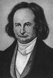
Charles Picard

If an initial position of the vector \( {\bf x} (t) \) is known, we get an initial value problem:

\begin{equation} \label{EqPicard.1} \frac{{\text d} {\bf x}}{{\text d}t} = {\bf f}(t, {\bf x} ) , \qquad {\bf x} (t_0 ) = {\bf x}_0 , \end{equation}
where \( {\bf x}_0 \) is an initial column vector. Many brilliant mathematicians participated in proving the existence of a solution to the given initial value problem more than 100 years ago. Their proof was based on what is now called the Picard's iteration, named after the French mathematician Charles Émile Picard (1856--1941) whose theories did much to advance research in analysis, algebraic geometry, and mechanics.

The Picard procedure is actually a practical extension of the Banach fixed point theorem, which is applicable to continuous contractible functions. Since any differential equation involves an unbounded derivative operator, the fixed point theorem is not suitable for it. To bypass this obstacle, Picard suggested to apply the (bounded) inverse operator L-1 to the first derivative \( \texttt{D} . \) Recall that the inverse \( \texttt{D}^{-1} , \) called in mathematical literature as «antiderivative», is not an operator because it assigns to every input-function infinite many outputs. To restrict its output to a single one, we consider the differential operator on the set of functions (which becomes a vector space only when the differential equation and the initial condition are all homogeneous) with a specified initial condition f(x0) = y0. So the derivative operator on this set of functions we denote by L, and its inverse is a bounded integral operator. The first step in deriving Picard's iterations is to rewrite the given initial value problem in equivalent (this is true when the slope function f is continuous in Lipschitz sense) form as Volterra integral equation of second kind:

\begin{equation} \label{EqPicard.2} {\bf x} ( t ) ={\bf x}_0 + \int_{t_0}^t {\bf f} (s, {\bf x} (s) ) \,{\text d}s . \end{equation}
This integral equation is obtained upon integration of both sides of the differential equation \( {\text d}{\bf x} / {\text d} t = {\bf f}(t, {\bf x}), \) subject to the initial condition.

The equivalence follows from the Fundamental Theorem of Calculus. It suffices to find a continuous function \( {\bf x}(t) \) that satisfies the integral equation within the interval \( t_0 -h < t < t_0 +h , \) for some small value \( h \) since the right hand-side (integral) will be continuously differentiable in \( t . \)

Assuming that the vector-function \( {\bf f} ({\bf x}, t) \) satisfies the Lipschitz condition in x:

\[ \| {\bf f}({\bf x} , t ) - {\bf f}({\bf y} ,t ) \| \le L\,\| {\bf x} - {\bf y} \| , \]
where constant L is called the Lipschitz constant, then the initial value problem \eqref{EqPicard.1} has a unique solution in some neighborhood of the initial position.

Now we apply a technique known as Picard iteration to construct the required solution:

\begin{equation} \label{EqPicard.3} {\bf x}_{m+1} ( t ) ={\bf x}_0 + \int_{t_0}^t {\bf f} (s, {\bf x}_m (s) ) \,{\text d}s , \qquad m=0,1,2,\ldots . \end{equation}
The initial approximation is chosen to be the initial value (constant): \( {\bf x}_0 (t) \equiv {\bf x}_0 .\) (The sign ≡ indicates the values are identically equivalent, so this function is the constant). When input function f(t, x) satisfies some (sufficient) conditions, it can be shown that this iterative sequence converges to the true solution uniformly on the interval \( [t_0 -h, t_0 +h ] \) when h is small enough. Actually, the necessary and sufficient conditions for existence of a solution to a vector initial value problem are still waiting for their discovery.

Of course, we can differentiate the recursive integral relation to obtain a sequence of the initial value problems

\begin{equation} \label{EqPicard.4} \frac{{\text d}{\bf x}_{m+1} ( t )}{{\text d}t} = {\bf f} (t, {\bf x}_m (t) , \qquad {\bf x}_m (t_0 ) = {\bf x}_0 , \qquad m=0,1,2,\ldots . \end{equation}
that is equivalent to the original recurrence \eqref{EqPicard.3}. However,this recurrence relation \eqref{EqPicard.4} involves the derivative operator \( \texttt{D} = {\text d}/{\text d}t . \) Since \( \texttt{D} \) is an unbounded operator, it is not possible to prove convergence of the iteration procedure \eqref{EqPicard.4}. On the other hand, the convergence of \eqref{EqPicard.3} involving a bounded integral operator can be accomplished directly (see Tutorial I).

Example 1: . Using Newton's laws of motion and gravitation you can in theory work out how a number of objects (say stars, planets and moons) should move due to the gravitational pull they exert on each other. If there are only two bodies involved the answer is straight-forward: they move along curves that are easy to describe (ellipses in the case of a planet orbiting a star). The problem of three or more bodies motivated the science community and Henri Poincaré solved this three body problem on November 30th 1889, unfortunately, withe a mistake. He revised his competition entry, still got the prize and was paid, and later wrote more extensively about what the mistake had revealed to him---the existence of chaos.

Let xij and vij represent the i-th position coordinate and the i-th velocity component, respectively, of particles j = 1, 2, …, N of respective masses mj. Furthermore, let \( r_{jk} = \left\vert \sum_{i=1}^3 \left( x_{ij} - x_{ik} \right)^2 \right\vert^{1/2} \) denote the separation distances between the centers of particles j and k, where k = 1, 2, …, N. In classical form, the N-body problem consists of 6N coupled autonomous first-order ODEs, namely \begin{equation*} \label{EqNbody.1} \begin{split} \frac{{\text d} x_{ij}}{{\text d}t} = v_{ij} , \\ \frac{{\text d} v_{ij}}{{\text d}t} = \sum_{k\ne j} m_k \left( x_{ik} - x_{ij} \right) / r_{jk}^3 . \end{split} \tag{1.1} \end{equation*} By defining the inverse separation distances to be \( s_{jk} = 1 / r_{jk} \ (j\ne k) , \) we derive the following polynomial formulation of the N-body problem: \begin{equation*} \label{EqNbody.2} \begin{cases} \frac{{\text d} x_{ij}}{{\text d}t} = v_{ij} , \\ \frac{{\text d} v_{ij}}{{\text d}t} = \sum_{k\ne j} m_k \left( x_{ik} - x_{ij} \right) * s_{jk}^3 , \\ \frac{{\text d} s_{ij}}{{\text d}t} = - s_{jk}^3 \sum_{i=1}^3 \left( x_{ik} - x_{ij} \right) \left( v_{ik} - v_{ij} \right) . \end{cases} \tag{1.2} \end{equation*} Even when symmetry is exploited ( \( s_{jk} = s_{kj} \) ), we have paid a price for polynomial form; the number of equations n has been increased to n = 6N +N(N - 1)/2. The gain is that the system now readily admits a Maclaurin-series solution of arbitrary order.

Let xijl denote the l-th order coefficient of the Maclaurin series for xij. That is, \( x_{ij}(t) = \sum_{l\ge 0} x_{ijl} t^l . \) Let similar notation hold for vij and sij. In light of the theoretical considerations mentioned previously, the coefficients for the m-th term are obtained simply by integrating (1.2) with respect to t, to yield \begin{equation*} \label{EqNbody.3} x_{ijm} = v_{i,j,m-1}/m . \tag{1.3} \end{equation*} Similarly, we have \begin{equation*} \label{EqNbody.4} v_{ijm} = \sum_{k=1}^n m_k \sum_{l=0}^{m-1} \left( x_{pkl} - x_{ijl} \right) \left( s^3 \right)_{j,k,m-l-1} /m , \tag{1.4} \end{equation*} where \begin{equation*} \label{EqNbody.5} \left( s^2 \right)_{jkm} = \sum_{l=0}^m s_{jkl} s_{j,k,l-m} , \qquad \left( s^3 \right)_{jkm} = \sum_{l=0}^m \left( s^2 \right)_{ijk} s_{j,k,l-m} \tag{1.5} \end{equation*} are convolutions of sequences s with itself. Finally, by defining \begin{equation*} \label{EqNbody.6} a_{jkm} = \sum_{l=1}^m \sum_{i=1}^3 \left( x_{ijl} - x_{ikl} \right) \left( v_{i,j,m-l} - v_{i,k,m-l} \right) , \tag{1.6} \end{equation*} we obtain from \begin{equation*} \label{EqNbody.7} s_{jkm} = - \sum_{l=1}^{m-1} \left( s^3 \right)_{jkl} a_{j,k,m-l} /m . \tag{1.7} \end{equation*}

The three-body problem with close encounters is notoriously ill-conditioned because it admits chaotic solutions that manifest extreme sensitivity to initial conditions. The following example demonstrates the Picard's method for an ill-conditioned three-body problem comprised of the earth, its moon,and a ‘‘spacecraft’’.

The numerical values of three body problem are presented in the following table. Data are only approximately related to realistic values. For all bodies, the initial coordinate x3 and velocity v3 are assumed zero so that the orbits remain co-planar. Masses are scaled relative to the mass of the earth; distances are in earth radii. Velocity is normalized by the orbital velocity at the earth's surface, for which the orbital period is 2π. The integration time (T = 3200) is in excess of 500 orbital periods.

 Body    Mass, Mj      x1      x2      v1      v2  
 Earth   1.0 0.0 0.0 0.0 0.0
 Moon   0.0125 42.4 −42.4 0.095 0.095
 Craft   0.00001 −1.0 0.0 0.0 1.4034
   ■


Picard's iteration for higher order differential equations


Now we turn our attention to applying Picard's iteration procedure to solving initial value problems for higher order (linear or nonlinear) single differential equations:
\begin{equation} \label{EqPicard.5} x^{(n)} (t) = f\left( t, x, x' , \ldots , x^{(n-1)} (t) \right) , \qquad x(0) = x_0 , \ x' (0) = x_1 , \ \ldots , \ x^{(n-1)} (0) = x_{n-1} , \end{equation}
where \( x^{(n)} (t) = \frac{{\text d}^n x}{{\text d}t^n} = \texttt{D}^n x(t) \) stands for the n-th derivative. There are usually two options to achieve this. First, we can transfer this single differential equation to an equivalent system of first order ODEs upon introducing new dependent variables:
\begin{equation} \label{EqPicard.6} y_1 (t) = x(t) , \quad y_2 (t) = x' (t) = y'_1 (t) , \quad \ldots , \quad y_{n} (t) = y'_{n-1} (t) = x^{(n-1)} (t) . \end{equation}
Rewriting this system of equations in a standard vector form \( \dot{\bf y} = {\bf f}(t, {\bf y}) , \) we can apply Picard's iterations for column-vector y.

Another approach is based on extension of Picard's idea for a higher order equation. It is based on the observation that the initial value problem for n-th order derivative

\begin{equation} \label{EqPicard.7} \texttt{D}^n x(t) = f(t, x, x' , \ldots , x^{(n-1)}) , \quad x(0) = x_0 , \ x' (0) = x_1 , \ \ldots , \ x^{(n-1)} (0) = x_{n-1} , \end{equation}
where \( \texttt{D} = \frac{{\text d}}{{\text d}t} \) is the derivative operator, has an explicit solution (which is unique)
\begin{equation} \label{EqPicard.8} x(t) = \frac{1}{(n-1)!} \int_0^t \left( t-s \right)^{n-1} f(s, x(s) , \ldots )\,{\text d}s + \sum_{k=0}^{n-1} \frac{x_k}{k!}\, t^k . \end{equation}
Upon denoting by ϕm(t) the m-th Picard iterate, we write the Picard iteration scheme:
\begin{equation} \label{EqPicard.9} \phi_{m+1} (t) = \frac{1}{(n-1)!} \int_0^t \left( t-s \right)^{n-1} f\left( s, \phi_m (s) , \ldots \right)\,{\text d}s + \sum_{k=0}^{n-1} \frac{a_{k}}{k!}\, t^k , \qquad m=0, 1, 2, \ldots , \end{equation}
where coefficients \( a_k \) and first n initial values of y and its derivatives at t = 0 to satisfy the initial conditions \eqref{EqPicard.5}. Since the convergence of the successive approximations to the true solution is often slow, it could be beneficial to choose the initial approximation wisely. All approaches are demonstrated in a series of examples.


Example 2: Consider the initial value problem for the first order differential equation

\[ \frac{{\text d}y}{{\text d}x} = \sqrt{\frac{1}{4} + 2\,y} , \qquad y(0) = 1. \tag{2.1} \]
We apply Picard's iteration directly by solving the fixed point problem
\[ \phi_{n+1} (x) = 1 + \int_0^x \sqrt{\frac{1}{4} + 2\,\phi_n (t)}\,{\text d}t , \qquad n=0,1,2,\ldots . \tag{2.2} \]
If we start with the initial condition ϕ0 = 1, we almost immediately come to a problem of explicit integration. Indeed, we calculate first the few terms:
\begin{align*} \phi_0 &= 1 , \\ \phi_1 (x) &= 1 +\int_0^x \sqrt{\frac{1}{4} + 2}\,{\text d}t = 1 + \frac{3}{2}\, x , \\ \phi_2 (x) &= 1 +\int_0^x \sqrt{\frac{1}{4} + 2\,\phi_1 (t)}\,{\text d}t = 1+ \int_0^x \sqrt{\frac{1}{4} + 2 +3\,t}\,{\text d}t = \frac{x}{\sqrt{3}}\, \sqrt{3 + 4\,x} + \frac{1}{4} \left( 1 + \sqrt{9 + 12\,x} \right) , \end{align*}
because Mathematica helps:
Simplify[1 + Assuming[x > 0, Integrate[Sqrt[9/4 + 3*t], {t, 0, x}]]]
x Sqrt[1 + (4 x)/3] + 1/4 (1 + Sqrt[9 + 12 x])
Although, the next iteration Mathematica can handle by invoking special functions,
Simplify[1 + Assuming[x > 0, Integrate[ Sqrt[t Sqrt[1 + (4 t)/3] + 1/4 (1 + Sqrt[9 + 12 t])], {t, 0, x}]]
it will not overcome the further step.


This example illustrates that Picard's scheme is not practical because the corresponding iteration cannot be performed indefinitely---the functions are not explicitly integrable. In order to apply Picard's method, the slope function must be a polynomial---otherwise the results of integration cannot be expressed through elementary functions. However, in many practical cases, this obstacle can be bypassed with introduction of auxiliary dependent variables and converting the given equation to a system of differential equations.

To apply Picard's method, we convert (see section) the given initial value problem to the system of differential equations upon introducing auxiliary dependent variables:

\begin{align*} y_1 (x) &= y(x), \\ y_2 (x) &= \sqrt{\frac{1}{4} + 2\,y(x)} , \\ y'_1 &= y_2 (x) , \\ y'_2 (x) &= \frac{1}{2\,\sqrt{\frac{1}{4} + 2\,y(x)}} \, 2\, y' (x) = 1 . \end{align*}
We get an equivalent to the given autonomous differential equation: a first order vector equation with a polynomial right-hand side input:
\[ \frac{\text d}{{\text d}x} \begin{bmatrix} y_1 (x) \\ y_2 (x) \end{bmatrix} = \begin{bmatrix} y_2 (x) \\ 1 \end{bmatrix} , \qquad \begin{bmatrix} y_1 (0) \\ y_2 (0) \end{bmatrix} = \begin{bmatrix} 1 \\ \frac{3}{2} \end{bmatrix} . \tag{2.3} \]
Integrating the vector equation above allows us to rewrite the given initial value problem in equivalent vector form:
\[ \begin{bmatrix} y_1 (x) \\ y_2 (x) \end{bmatrix} = \begin{bmatrix} 1 \\ \frac{3}{2} \end{bmatrix} + \int_0^x \begin{bmatrix} y_2 (s) \\ 1 \end{bmatrix} {\text d} s . \]
The Picard's iteration scheme will be
\[ \begin{bmatrix} \phi_1 (x) \\ \phi_2 (x) \end{bmatrix}_{(m+1)} = \begin{bmatrix} 1 \\ \frac{3}{2} \end{bmatrix} + \int_0^x \begin{bmatrix} \phi_2 (s) \\ 1 \end{bmatrix}_{(m)} {\text d} s , \qquad m=0,1,2, \ldots . \]
Since Picard's iteration always starts with the initial condition, we get
\[ \begin{bmatrix} \phi_1 (x) \\ \phi_2 (x) \end{bmatrix}_{(1)} = \begin{bmatrix} 1 \\ \frac{3}{2} \end{bmatrix} + \int_0^x \begin{bmatrix} \frac{3}{2} \\ 1 \end{bmatrix} {\text d} s = \begin{bmatrix} 1 \\ \frac{3}{2} \end{bmatrix} + \begin{bmatrix} \frac{3}{2}\, x \\ x \end{bmatrix} = \begin{bmatrix} 1+\frac{3}{2}\, x \\ \frac{3}{2} + x \end{bmatrix} . \]
Next term will be
\[ \begin{bmatrix} \phi_1 (x) \\ \phi_2 (x) \end{bmatrix}_{(2)} = \begin{bmatrix} 1 \\ \frac{3}{2} \end{bmatrix} + \int_0^x \begin{bmatrix} \frac{3}{2} +s \\ 1 \end{bmatrix} {\text d} s = \begin{bmatrix} 1+ \frac{3}{2}\, x + \frac{x^2}{2} \\ \frac{3}{2} +x \end{bmatrix} . \]
The second component, ϕ2, remains the same with every iteration. This component is used to generate the first component, ϕ1, as well. As such, every following iteration will be the same, and the true solution becomes
\[ y(x) = 1 +\frac{3}{2}\, x + \frac{x^2}{2} . \]
Its derivative is
\[ y' (x) = \frac{3}{2} + x \qquad \Longrightarrow \qquad \frac{1}{4} + 2\, y(x) = \left( \frac{3}{2} + x \right)^2 . \]
   ■

Example 3: Consider the initial value problem for the simple pendulum equation

\[ \frac{{\text d}^2 \theta}{{\text d} t^2} + \sin \theta = 0 , \qquad \theta (0) = \frac{\pi}{4} , \quad \dot{\theta} (0) = \frac{1}{10} , \tag{3.1} \]
where dot stands for the derivative with respect to time variable t. We integrate the pendulum equation above twice, and use initial condition provided. We may try to apply Picard's iteration scheme
\[ \phi_{m+1} (t) = \frac{\pi}{4} + \frac{1}{10}\, t - \int_0^t \left( t-s \right) \sin \phi_m (s) \,{\text d}s , \qquad m= 0,1,2, \ldots . \tag{3.2} \]
The initial function is chosen to match the initial conditions: \( \phi_{0} (t) = \frac{\pi}{4} + \frac{t}{10} . \) Although we can find the next term
\[ \phi_{1} (t) = \frac{\pi}{4} + \frac{1}{10}\, t - \int_0^t \left( t-s \right) \sin \left( \frac{\pi}{4} + \frac{1}{10}\,s \right) {\text d}s = \frac{\pi}{4} + \frac{1}{10}\, t + 5\sqrt{2} \left( 10 +t \right) - 100\,\sin \frac{5\pi + 2t}{20} \]
with the aid of Mathematica
Simplify[Pi/4 + t/10 + Assuming[t > 0, Integrate[(t - s)*Sin[Pi/4 + s/10], {s, 0, t}]]]
the second term ϕ2(t) is impossible to determine, even for such a powerful computer algebra system as Mathematica. We can bypass this obstacle by introducing auxiliary variables:
\begin{align*} y_1 (t) &= \theta (t), \\ y_2 (t) &= \dot{y}_1 = \dot{\theta} , \\ y_3 (t) &= \sin \theta (t) , \\ y_4 (t) &= \cos \theta (t) . \end{align*}
Then the pendulum equation and corresponding initial conditions will be equivalent to the following IVP:
\[ \frac{\text d}{{\text d}t} \begin{bmatrix} y_1 (t) \\ y_2 (t) \\ y_3 (t) \\ y_4 (t) \end{bmatrix} = \begin{bmatrix} y_2 (t) \\ -y_3 (t) \\ y_2 (t)\,y_4 (t) \\ -y_2 (t)\,y_3 (t) \end{bmatrix} , \qquad \begin{bmatrix} y_1 (0) \\ y_2 (0) \\ y_3 (0) \\ y_4 (0) \end{bmatrix} = \begin{bmatrix} \frac{\pi}{4} \\ \frac{1}{10} \\ \frac{1}{\sqrt{2}} \\ \frac{1}{\sqrt{2}} \end{bmatrix} . \tag{3.3} \]
Since this system of four differential equations has a polynomial slope part, we expect to perform all steps of Picard's iteration scheme:
\[ \begin{bmatrix} \phi_1 (t) \\ \phi_2 (t) \\ \phi_3 (t) \\ \phi_4 (t) \end{bmatrix}_{(m+1)} = \begin{bmatrix} \frac{\pi}{4} \\ \frac{1}{10} \\ \frac{1}{\sqrt{2}} \\ \frac{1}{\sqrt{2}} \end{bmatrix} + \int_0^t \begin{bmatrix} \phi_2 (t) \\ -\phi_3 (t) \\ \phi_2 (t)\,\phi_4 (t) \\ -\phi_2 (t)\,\phi_3 (t) \end{bmatrix}_{(m)} {\text d} s , \qquad m=0,1,2,\ldots . \tag{3.4} \]
The first term is
\[ \begin{bmatrix} \phi_1 (t) \\ \phi_2 (t) \\ \phi_3 (t) \\ \phi_4 (t) \end{bmatrix}_{(1)} = \begin{bmatrix} \frac{\pi}{4} \\ \frac{1}{10} \\ \frac{1}{\sqrt{2}} \\ \frac{1}{\sqrt{2}} \end{bmatrix} + \int_0^t \begin{bmatrix} \frac{1}{10} \\ -\frac{1}{\sqrt{2}} \\ \frac{1}{10} \,\frac{1}{\sqrt{2}} \\ -\frac{1}{10} \,\frac{1}{\sqrt{2}} \end{bmatrix} {\text d} s = \begin{bmatrix} \frac{\pi}{4} \\ \frac{1}{10} \\ \frac{1}{\sqrt{2}} \\ \frac{1}{\sqrt{2}} \end{bmatrix} + t \begin{bmatrix} \frac{1}{10} \\ -\frac{1}{\sqrt{2}} \\ \frac{1}{10} \,\frac{1}{\sqrt{2}} \\ -\frac{1}{10} \,\frac{1}{\sqrt{2}} \end{bmatrix} . \]
Next,
\[ \begin{bmatrix} \phi_1 (t) \\ \phi_2 (t) \\ \phi_3 (t) \\ \phi_4 (t) \end{bmatrix}_{(2)} = \begin{bmatrix} \frac{\pi}{4} \\ \frac{1}{10} \\ \frac{1}{\sqrt{2}} \\ \frac{1}{\sqrt{2}} \end{bmatrix} + \int_0^t \begin{bmatrix} \frac{1}{10} - \frac{s}{\sqrt{2}} \\ -\frac{1}{\sqrt{2}} + \frac{s}{10\,\sqrt{2}} \\ \left( \frac{-s}{\sqrt{2}} + \frac{1}{10} \right) \left( \frac{1}{\sqrt{2}} + \frac{s}{10\,\sqrt{2}} \right) \\ -\left( \frac{-s}{\sqrt{2}} + \frac{1}{10} \right) \left( \frac{1}{\sqrt{2}} - \frac{s}{10\,\sqrt{2}} \right) \end{bmatrix} {\text d} s = \begin{bmatrix} \frac{\pi}{4} \\ \frac{1}{10} \\ \frac{1}{\sqrt{2}} \\ \frac{1}{\sqrt{2}} \end{bmatrix} + \begin{bmatrix} \frac{t}{10} - \frac{t^2}{2\,\sqrt{2}} \\ -\frac{t}{\sqrt{2}} + \frac{t^2}{20\,\sqrt{2}} \\ \frac{t}{10\,\sqrt{2}} - \frac{t^2}{4} + \frac{t^2}{200\,\sqrt{2}} - \frac{t^3}{60} \\ -\frac{t}{10\,\sqrt{2}} + \frac{t^2}{4} - \frac{t^2}{200\,\sqrt{2}} - \frac{t^3}{60} \end{bmatrix} . \]
-(1/Sqrt[2] + t/10/Sqrt[2])*(1/10 - t/Sqrt[2])
-(1/(10 Sqrt[2])) + t/2 - t/(100 Sqrt[2]) + t^2/20
(1/Sqrt[2] - t/10/Sqrt[2])*(1/10 - t/Sqrt[2])
Expand[%]
1/(10 Sqrt[2]) - t/2 - t/(100 Sqrt[2]) + t^2/20
We can expand this procedure indefinitely and obtain
\[ \theta (t) = \frac{\pi}{4} + \frac{t}{10} -\frac{\sqrt{2}}{4}\, t^2 - \frac{\sqrt{2}}{120}\, t^3 + \left( \frac{1}{48} + \frac{\sqrt{2}}{4800} \right) t^4 + \left( \frac{\sqrt{2}}{240 000} - \frac{1}{1200} \right) t^5 + \left( \frac{1111\,\sqrt{2}}{1600 000} - \frac{11}{144 000} \right) t^6 + \cdots . \]
We check our answer with Mathematica:
AsymptoticDSolveValue[{theta''[t] + Sin[theta[t]] == 0, theta[0] == Pi/4, theta'[0] == 1/10}, theta[t], {t, 0, 7}]
\[Pi]/4 + t/10 - t^2/(2 Sqrt[2]) - t^3/( 60 Sqrt[2]) + ((100 + Sqrt[2]) t^4)/4800 + ((-200 + Sqrt[ 2]) t^5)/240000 + ( 11 (-100 + 909 Sqrt[2]) t^6)/14400000 + ((400 + 159999 Sqrt[2]) t^7)/1008000000
      Now we plot Picard's polynomial approximation along with a true solution.
theta6[t_] = \[Pi]/4 + t/10 - t^2/(2 Sqrt[2]) - t^3/( 60 Sqrt[2]) + ((100 + Sqrt[2]) t^4)/4800 + ((-200 + Sqrt[2]) t^5)/ 240000 + (11 (-100 + 909 Sqrt[2]) t^6)/14400000;
s = NDSolve[{x''[t] + Sin[x[t]] == 0, x[0] == Pi/4, x'[0] == 1/10}, x, {t, 0, 8}];
Plot[{Callout[theta6[t], "Picard", LabelStyle -> Medium], Callout[x[t] /. s, "true", LabelStyle -> Medium]}, {t, 0, 5.0}, PlotTheme -> "Business"]
       Figure 1: Picard's approximation along with the true solution.            Mathematica code

   ■

Example 4: Let us apply Picard's iteration procedure to a constant coefficient homogeneous vector differential equation

\[ \dot{\bf x} (t) = {\bf A}\, {\bf x}(t) , \qquad {\bf x}(0) = {\bf x}_0 , \tag{4.1} \]
where A is n × n constant matrix and x(t) is unknown n-column vector. First, we transfer the given initial value problem to the integral equation
\[ {\bf x}(t) = {\bf x}_0 + \int_0^t {\bf A}\, {\bf x}(s)\,{\text d}s = {\bf x}_0 + {\bf A} \int_0^t {\bf x}(s)\,{\text d}s . \tag{4.2} \]
Note that matrix A is constant, so we can exchange the order of integration and multiplication by matrix A. Now we employ Picard's iteration scheme:
\[ {\bf \phi}_{m+1} (t) = {\bf x}_0 + {\bf A} \int_0^t {\bf \phi}_m (s)\,{\text d}s . \tag{4.3} \]
To start iteration, we have to choose the initial value \( {\bf \phi}_0 = {\bf x}_0 . \) Otherwise, the integral equation will be not equivalent to the given initial value problem. Then next iteration will be
\[ {\bf \phi}_1 = {\bf x}_0 + \int_0^t {\bf A}\, {\bf x}_0 \,{\text d}s = {\bf x}_0 + {\bf A}\,\int_0^t {\bf x}_0 \,{\text d}s = {\bf x}_0 + {\bf A}\,t \, {\bf x}_0 = {\bf x}_0 + t\,{\bf A} \, {\bf x}_0 . \]
The second term will be
\[ {\bf \phi}_2 = {\bf x}_0 + \int_0^t {\bf A}\, {\bf x}_1 \,{\text d}s = {\bf x}_0 + {\bf A}\,\int_0^t \left( {\bf x}_0 + {\bf A}\,s \right) {\text d}s = {\bf x}_0 + t\, {\bf A}\,{\bf x}_0 + \frac{t^2}{2} \, {\bf A}^2 {\bf x}_0 . \]
The third term becomes
\[ {\bf \phi}_3 = {\bf x}_0 + \int_0^t {\bf A}\, {\bf x}_2 \,{\text d}s = {\bf x}_0 + {\bf A}\,\int_0^t \left( {\bf x}_0 + {\bf A}\,s + {\bf A}^2 \frac{s^2}{2} \right) {\text d}s = {\bf x}_0 + t\, {\bf A}\,{\bf x}_0 + \frac{t^2}{2} \, {\bf A}^2 {\bf x}_0 + \frac{t^3}{2\cdot 3} \, {\bf A}^3 {\bf x}_0 . \]
The pattern is obvious and we can write the n-th iterate as
\[ {\bf \phi}_n (t) = {\bf x}_0 + t\, {\bf A}\,{\bf x}_0 + \frac{t^2}{2} \, {\bf A}^2 {\bf x}_0 + \cdots + \frac{t^n}{n!} \, {\bf A}^n {\bf x}_0 . \tag{4.4} \]
E. Picard proved that the sequence of n-column vector functions ϕm(t) converges to the solution x>(t) of the given IVP as m → ∞. From the explicit formula for ϕm(t), it follows that it is the m-th approximation of the exponential matrix function:
\[ e^{{\bf A}\,t} = {\bf I} + t\,{\bf A} + \frac{t^2 {\bf A}^2}{2!} + \cdots + \frac{t^m {\bf A}^m}{m!} + \cdots . \tag{4.5} \]
Since matrix A is constant, the series for the exponential matrix converges for every real t.    ■

Example 5: . Let us consider the system of differential equations subject to the initial conditions

\[ \begin{split} \dot{x} &= -6\,x + 4\,y , \\ \dot{y} &= \phantom{-}5\,x -5\,y ; \end{split} \qquad x(0) = 2, \quad y(0) =0 . \tag{5.1} \]
Of course, Mathematica knows how to solve it:
DSolve[{x'[t] == -6*x[t] + 4*y[t], y'[t] == 5*x[t] - 5*y[t], x[0] == 2, y[0] == 0}, {x[t], y[t]}, t]
{{x[t] -> 2/9 E^(-10 t) (5 + 4 E^(9 t)), y[t] -> 10/9 E^(-10 t) (-1 + E^(9 t))}}
\[ x(t) = \frac{10}{9}\, e^{-10t} + \frac{8}{9}\, e^{-t} , \qquad y(x) = - \frac{10}{9}\, e^{-10t} + \frac{10}{9}\, e^{-t} . \]
We convert the given IVP into the integral equation:
\[ \begin{bmatrix} x(t) \\ y(t) \end{bmatrix} = \begin{bmatrix} 2 \\ 0 \end{bmatrix} + \int_0^t \begin{bmatrix} -6\,x(s) + 4\,y(s) \\ 5\,x(s) -5\,y(s) \end{bmatrix} {\text d} s = \begin{bmatrix} 2 \\ 0 \end{bmatrix} + \begin{bmatrix} -6&\phantom{-}4 \\ \phantom{-}5 & -5 \end{bmatrix} \int_0^t \begin{bmatrix} x(s) \\ y(s) \end{bmatrix} {\text d} s . \tag{5.2} \]
It is useful, but not necessary to rewrite the system of ODEs (5.1) as a single second order differential equation
\[ \ddot{z} + 11\,\dot{z} + 10\, z =0, \qquad z(0) =2, \quad \dot{z} (0) =-22 , \tag{5.3} \]
where z = xy. This leads to the following integral equation
\[ z(t) = 2-22t - \int_0^t \left( t-s \right) \left[ 11\,\dot{z} + 10\,z(s) \right] {\text d}s . \]
Integrating by parts, we obtain
\[ z(t) = 2 - \int_0^t \left[ 11 + 10 \left( t-s \right) \right] z(s)\, {\text d}s . \tag{5.4} \]
Eq.(5.4) is used to generate Picard's iterations:
\[ z_{m+1} (t) = 2 - \int_0^t \left[ 11 + 10 \left( t-s \right) \right] z_m (s)\, {\text d}s . \tag{5.5} \]
First, we solve the initial value problem with Mathematica
DSolve[{10 z[t] + 11 Derivative[1][z][t] + (z^\[Prime]\[Prime])[t] == 0, z[0] == 2, Derivative[1][z][0] == -22}, z[t], t]
{{z[t] -> -(2/9) E^(-10 t) (-10 + E^(9 t))}}
\[ z(t) = \frac{20}{9}\, e^{-10t} - \frac{2}{9}\, e^{-t} . \]
Expanding this solution into Taylor's series, we obtain
\[ z(t) = 2 - 22\,t + 111\,t^2 - \frac{1111}{3}\, t^3 + \frac{11111}{12}\, t^4 - \frac{37037}{20}\,t^5 + \frac{1111111}{360}\, t^6 - \cdots . \]
Series[20/9 Exp[-10*t] - 2/9*Exp[-t], {t, 0,
SeriesData[t, 0, {2, -22, 111, Rational[-1111, 3], Rational[11111, 12], Rational[-37037, 20], Rational[1111111, 360], Rational[-11111111, 2520], Rational[12345679, 2240]}, 0, 9, 1]
Now we apply iteration scheme (5.4) and obtain some approximations:
z[0][t_] =2;
z[1][t_] = 2 - Integrate[(11 + 10*(t - s))*z[0][s], {s, 0, t}]
2 - 22 t - 10 t^2
z[2][t_] = 2 - Integrate[(11 + 10*(t - s))*z[1][s], {s, 0, t}]
2 - 22 t + 111 t^2 + (220 t^3)/3 + (25 t^4)/3
z[3][t_] = 2 - Integrate[(11 + 10*(t - s))*z[2][s], {s, 0, t}]
2 - 22 t + 111 t^2 - (1111 t^3)/3 - (1765 t^4)/6 - 55 t^5 - (25 t^6)/9
z[4][t_] = 2 - Integrate[(11 + 10*(t - s))*z[3][s], {s, 0, t}]
2 - 22 t + 111 t^2 - (1111 t^3)/3 + (11111 t^4)/12 + (2497 t^5)/3 + ( 1790 t^6)/9 + (1100 t^7)/63 + (125 t^8)/252
z[5][t_] = 2 - Integrate[(11 + 10*(t - s))*z[4][s], {s, 0, t}]
2 - 22 t + 111 t^2 - (1111 t^3)/3 + (11111 t^4)/12 - ( 37037 t^5)/20 - (22015 t^6)/12 - (3575 t^7)/7 - (1250 t^8)/21 - ( 6875 t^9)/2268 - (125 t^10)/2268
So the sixth iterate becomes
\[ z_6 (t) = 2 - 22\,t + 111\,t^2 - \frac{1111}{3}\, t^3 + \frac{11111}{12}\, t^4 - \frac{37037}{20}\,t^5 + \frac{1111111}{360}\, t^6 - \frac{19943}{6}\, t^7 + \cdots . \]
      Now we plot 6-th Picard's polynomial approximation along with a true solution z(t).
phi6[t_] = 2 - 22 t + 111 t^2 - (1111 t^3)/3 + (11111 t^4)/12 - (37037 t^5)/ 20 + (1111111 t^6)/360 + (19943 t^7)/6 + (346025 t^8)/336 + ( 108625 t^9)/756 + (45125 t^10)/4536 + (125 t^11)/378 + (625 t^12)/ 149688;
z[t_] = 20/9 Exp[-10*t] - 2/9*Exp[-t];
Plot[{Callout[phi6[t], "Picard", LabelStyle -> Medium], Callout[z[t], "true", LabelStyle -> Medium]}, {t, 0, 0.33}, PlotTheme -> "Business"]
       Figure 6a: Picard's approximation ϕ6(t) along with the true solution z(t).            Mathematica code

We can express variables x and y through z:
\[ \dot{z} = \dot{x} - \dot{y} = -6 \,x + 4\,y - 5\,x + 5\,y = -11\,x + 9\,y . \]
Upon solving this system of algebraic equations, we get
\[ \begin{split} z &= x-y , \\ \dot{z} &= -11\,x + 9\,y . \end{split} \]
Mathematica helps:
Solve[{z == x - y, zdot == -11*x + 9*y}, {x, y}]
{{x -> 1/2 (-9 z - zdot), y -> 1/2 (-11 z - zdot)}}
This yields
\[ x = - \frac{1}{2} \left( 9\, z + \dot{z} \right) \qquad\mbox{and}\qquad y = - \frac{1}{2} \left( 11\, z + \dot{z} \right) . \]
Picard's iteration for system (5.1) becomes
\[ \begin{bmatrix} x(t) \\ y(t) \end{bmatrix}_{(m+1)} = \begin{bmatrix} 2 \\ 0 \end{bmatrix} + \int_0^t \begin{bmatrix} -6\,x(s) + 4\,y(s) \\ 5\,x(s) - 5\,y(s) \end{bmatrix}_{(m)} \,{\text d}s , \qquad m=0,1,2,\ldots . \tag{5.6} \]
Calculating the first few iterations, we obtain
\[ \begin{split} \begin{bmatrix} x (t) \\ y(t) \end{bmatrix}_{(1)} &= \begin{bmatrix} 2 \\ 0 \end{bmatrix} + \int_0^t \begin{bmatrix} -6\,x(0) + 4\,y(0) \\ 5\,x(0) - 5\,y(0) \end{bmatrix} = \begin{bmatrix} 2 - 12\,t \\ 10\,t \end{bmatrix} , \\ \begin{bmatrix} x (t) \\ y(t) \end{bmatrix}_{(2)} &= \begin{bmatrix} 2 \\ 0 \end{bmatrix} + \int_0^t \begin{bmatrix} -6\,x_1 (s) + 4\,y_1 (s) \\ 5\,x_1 (s) - 5\,y_1 (s) \end{bmatrix} = \begin{bmatrix} 2 - 12\,t + 56\, t^2 \\ 10\,t - 55\, t^2 \end{bmatrix} , \\ \begin{bmatrix} x (t) \\ y(t) \end{bmatrix}_{(3)} &= \begin{bmatrix} 2 - 12\,t + 56\, t^2 - \frac{556}{3}\, t^3 \\ 10\,t - 55\, t^2 + 185\, t^3 \end{bmatrix} . \end{split} \]
Using the single differential equation, we have
\[ \phi_{m+1} (t) = 2 -22t - \int_0^t \left( t-s \right) \left[ 11\,\phi'_m (s) + 10\,\phi_m (s) \right] {\text d} s, \qquad \phi_0 = 2, \quad \dot{\phi}_0 = -22 , \qquad m=0,1,2,\ldots . \]
Again, the first few iterations are
\[ \begin{split} \phi_1 (t) &= 2 - 22\,t + 111\,t^2 \qquad \Longrightarrow \qquad \dot{\phi}_1 = -22 + 222\, t , \\ \phi_2 (t) &= 2 - 22\,t + 111\,t^2 - \frac{1111}{3}\, t^3 - \frac{185}{2}\, t^4 \qquad \Longrightarrow \qquad \dot{\phi}_1 = -22 + 222\, t - 1111\, t^2 - 370\, t^3 , \\ \phi_3 (t) &= 2 - 22\,t + 111\,t^2 - \frac{1111}{3}\, t^3 - \frac{185}{2}\, t^4 \qquad \Longrightarrow \qquad \dot{\phi}_1 = -22 + 222\, t - 1111\, t^2 - 370\, t^3 . \end{split} \]
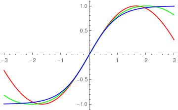
As we see, single equation iteration is faster than the previous. We can compare our single equation iteration with Picard's scheme for the original system of first order equations:
\[ x_1 = - \frac{1}{2} \left( 9\, \phi_1 + \dot{\phi}_1 \right) = -2 + 12\,t + \frac{999}{2}\, t^2 \]

Based on the single differential equation \( \ddot{z} + 11\,\dot{z} + 10\, z =0, \) we transfer it to the system of first order equations using standard substitutions:

\[ \dot{z} = u, \qquad \dot{u} = -11\, u -10\, z . \]
This leads to the following Picard's scheme:
\[ \begin{bmatrix} z(t) \\ u(t) \end{bmatrix}_{(m+1)} = \begin{bmatrix} 2 \\ -22 \end{bmatrix} + \int_0^t \begin{bmatrix} u(s) \\ -11\,u(s) - 10\,z(s) \end{bmatrix}_{(m)} {\text d}s , \qquad m=0,1,2,\ldots . \]
A first few terms are
\[ \begin{split} \begin{bmatrix} z(t) \\ u(t) \end{bmatrix}_{(1)} &= \begin{bmatrix} 2 - 22\,t \\ -22 + 222\,t \end{bmatrix} , \\ \begin{bmatrix} z(t) \\ u(t) \end{bmatrix}_{(2)} &= \begin{bmatrix} 2 - 22\,t + 111\,t^2 \\ -22 + 222\,t - 1111\,t^2 \end{bmatrix} , \\ \begin{bmatrix} z(t) \\ u(t) \end{bmatrix}_{(3)} &= \begin{bmatrix} 2 - 22\,t + 111\,t^2 - \frac{1111}{3}\,t^3 \\ -22 + 222\,t - 1111\,t^2 - \frac{11111}{3}\, t^3 \end{bmatrix} . \end{split} \]
   ■

Example 6: The objective of this example is to demonstrate that Picard's method generates noise terms along with true approximations when applied to a differential equation with variable coefficients. Of course, these noise terms are eliminated with next iteration, but new and less significant noise terms appear.

Consider the initial value problem:

\[ \frac{{\text d}^2 y}{{\text d}x^2} + 2x\, \frac{{\text d}y}{{\text d}x} - 2\,y(x) =0 , \qquad y(0) =1, \quad y' (0) = -1. \tag{6.1} \]
Its solution according to Mathematica is
DSolve[{y''[t] + 2*t*y'[t] - 2*y[t] == 0, y[0] == 1, y'[0] == -1}, y[t], t]
{{y[t] -> E^-t^2 (1 - E^t^2 t + E^t^2 Sqrt[\[Pi]] t Erf[t])}}
\[ y(x) = e^{-x^2 /2} -x + x\, \sqrt{\pi} \,\mbox{erf}(x) = e^{-t^2 /2} -x + 2\,x\,\int_0^x e^{-t^2 /2} \,{\text d}t , \tag{6.2} \]
where erf(x) = \( \frac{2}{\sqrt{\pi}} \, \int_0^x e^{-t^2 /2} \,{\text d}t \) is the error function. Before applying Picard's iteration scheme, we find its Maclaurin approximation:
\[ y(x) = 1 - x + x^2 - \frac{x^4}{6} + \frac{x^6}{30} - \frac{x^8}{168} + \frac{x^{10}}{1080} - \frac{x^{12}}{7920} + \cdots . \tag{6.3} \]
We need this expansion to check the quality of Picard's iterations. This is where Mathematica is extremely helpful; to achieve this, you have two options: use either Series or AsymptoticDSolveValue command. We apply the latter:
AsymptoticDSolveValue[{y''[x] + 2*x*y'[x] - 2*y[x] == 0, y[0] == 1, y'[0] == -1}, y[x], {x, 0, 10}]
1 - x + x^2 - x^4/6 + x^6/30 - x^8/168 + x^10/1080
The given differential equation has a Maclaurin power series solution that converges everywhere in ℂ because its coefficients are holomorphic functions:
\[ y(x) = 1 - x + \sum_{n\ge 2} c_n x^n . \]
The linear term 1−x is chosen to satisfy the initial conditions, and coefficients cn are to be determined from the equation. Its derivatives are
\[ y'(x) = -1 + \sum_{n\ge 2} c_n n\, x^{n-1} , \qquad y'' (x) = \sum_{n\ge 2} c_n n \left( n-1 \right) x^{n-2} = \sum_{k\ge 0} c_{k+2} \left( k+2 \right) \left( k+1 \right) x^k . \]
Substitution into the given differential equation yields
\begin{align*} y'' + 2x\,y' -2\,y &= \sum_{k\ge 0} c_{k+2} \left( k+2 \right) \left( k+1 \right) x^k -2x + 2 \sum_{n\ge 2} c_n n\, x^{n} -2 + 2x - 2\sum_{n\ge 2} c_n x^n \\ &= 2 \left( c_2 -1 \right) + 6x \,c_3 + \sum_{n\ge 2} \left[ c_{n+2} \left( n+2 \right) \left( n+1 \right) + 2c_n n - 2\,c_n\right] x^n = 0. \end{align*}
Equating coefficients of like powers of x, we obtain the recurrence:
\[ c_{n+2} = \frac{2 - 2n}{\left( n+2 \right) \left( n+1 \right)} c_n = - \frac{2\left( n-1 \right)}{\left( n+2 \right) \left( n+1 \right)} \, c_n , \qquad n=2,3,\ldots ; \]
where the first two terms are
\[ c_2 = 1 , \qquad c_3 = 0. \]
Thus, we obtain the convergent power series solution
\[ y(x) = 1 - x + x^2 - \frac{x^4}{6} + \frac{x^5}{30} - \frac{x^8}{168} + \cdots . \]
   ▣

First, we transfer the given problem to the system of first order differential equations by introducing new variables: y1 = y(x) and y2 to be its derivative. Then we get

\[ \frac{\text d}{{\text d}x}\,{\bf y} \equiv \frac{\text d}{{\text d}x} \begin{bmatrix} y_1 \\ y_2 \end{bmatrix} = \begin{bmatrix} y_2 \\ 2\,y_1 - 2x\, y_2 \end{bmatrix} \qquad \Longleftrightarrow \qquad \begin{split} y'_1 &= y_2 , \\ y'_2 &= 2\, y_1 -2x\,y_2 . \end{split} \tag{6.4} \]
Starting with the initial condition as the first approximation, we obtain the Picard's iteration formula:
\[ \phi_{m+1} (x) \equiv \begin{bmatrix} y_1 (x) \\ y_2 (x) \end{bmatrix}_{(m+1)} = \begin{bmatrix} \phantom{-}1 \\ -1 \end{bmatrix} + \int_0^x \begin{bmatrix} y_2 (t) \\ 2\, y_1 (t) -2t\,y_2 (t) \end{bmatrix}_{(m)} {\text d}t , \qquad \phi_0 = \begin{bmatrix} \phantom{-}1 \\ -1 \end{bmatrix} . \tag{6.5} \]
The third approximation ϕ3 has noise terms of order four. Of course, they will be eliminated with next iterations, but new ones of higher degree appear with every iterative step. This is typical for Picard's iterations because the given differential equation has variable coefficients. Noise terms are not observed only for autonomous differential equations.


Now we calculate some first iterations directly from the second order differential equation without converting it to a system of first order equations. Integrating twice both sides of the given differential equation, we obtain
\[ y(x) = 1 - x + \int_0^t {\text d}t \int_0^t \left[ - 2y' (s) + 2y(s) \right] {\text d}s . \]
Upon exchanging the order of integration, we get
\[ \int_0^t {\text d}t \int_0^t \left[ - 2y' (s) + 2y(s) \right] {\text d}s = \int_0^t \left[ - 2y' (s) + 2y(s) \right] {\text d}s \int_s^t {\text d}t = \int_0^t \left( t-s \right)\left[ - 2y' (s) + 2y(s) \right] {\text d}s . \]
The corresponding Picard's scheme becomes
\[ \phi_{(m+1)} (x) = 1-x + \int_0^x \left( x- s \right) \left[ 2\,\phi_{(m)} (s) - 2s\,\phi'_{(m)} (s) \right] {\text d}s , \qquad m=0,1,2,\ldots . \]
We can simplify this scheme further by eliminating the derivative of the unknown function under the sign of integral. Integrating by parts the term containing the derivative of ϕm, we reduce Picard's scheme to the following
\[ \phi_{(m+1)} (x) = 1-x + 2 \int_0^x \left( 2x- 3s \right) \phi_{(m)} (s)\, {\text d}s , \qquad m=0,1,2,\ldots . \tag{6.6} \]
For[{n = 1, y[0][x_] = {1, -1}}, n < 4, n++, y[n][x_] = {1, -1} + Integrate[{y[n - 1][t][[2]], 2*y[n - 1][t][[1]] - 2*t*y[n - 1][t][[2]]}, {t, 0, x}]];
Do[Print["n= ", n, " y(n)= ", y[n][x]], {n, 0, 3}]
n= 0 y(n)= {1,-1}
n= 1 y(n)= {1-x,-1+2 x+x^2}
n= 2 y(n)= {1-x+x^2+x^3/3,-1+2 x-(4 x^3)/3-x^4/2}
n= 3 y(n)= {1-x+x^2-x^4/3-x^5/10,-1+2 x-(2 x^3)/3+x^4/6+(8 x^5)/15+x^6/6}
So we get the third approximation to be
\[ \phi_3 (x) = 1 - x + x^2 - \frac{x^4}{3} - \frac{x^5}{10} , \]
which we compare with the true solution, obtained with the aid of Maclaurin expansion
Series[E^-t^2 (1 - E^t^2 t + E^t^2 Sqrt[\[Pi]] t Erf[t]), {t, 0, 6}]
SeriesData[t, 0, {1, -1, 1, 0, Rational[-1, 6], 0, Rational[1, 30]}, 0, 7, 1]
\[ y(x) = 1 - x + x^2 - \frac{x^4}{3} + \frac{x^6}{30} + \cdots . \]

If you do not trust our iteration code, you can check manually step by step. Upon choosing the initial term in accordance to the initial conditions

\[ \phi_{(0)} (x) = 1-x , \]
we find the first iterate:
\[ \phi_{(1)} (x) = 1-x + 2 \int_0^x \left( 2x- 3s \right) \left( 1 - s \right) \, {\text d}s = 1-x+x^2 \]
2*Integrate[(2*x-3*s)*(1-s),{s,0,x}]
x^2
The next iteration gives
\[ \phi_{(2)} (x) = 1-x + 2 \int_0^x \left( 2x- 3s \right) \left( 1 - s - s^2 \right) \, {\text d}s = 1-x+x^2 - \frac{x^4}{6} , \]
and so on. Instead of looping, we demonstrate each Picard's iterative step:
phi[0][x_] = 1 - x;
phi[1][x_] = phi[0][x] + 2 Integrate[(2*x - 3*s)*phi[0][s], {s, 0, x}]
1 - x + x^2
phi[2][x_] = phi[0][x] + 2 Integrate[(2*x - 3*s)*phi[1][s], {s, 0, x}]
1 - x + 2 (x^2/2 - x^4/12)
phi[3][x_] = phi[0][x] + 2 Integrate[(2*x - 3*s)*phi[2][s], {s, 0, x}]
1 - x + 2 (x^2/2 - x^4/12 + x^6/60)
phi[4][x_] = phi[0][x] + 2 Integrate[(2*x - 3*s)*phi[3][s], {s, 0, x}]
1 - x + 2 (x^2/2 - x^4/12 + x^6/60 - x^8/336)
phi[5][x_] = phi[0][x] + 2 Integrate[(2*x - 3*s)*phi[4][s], {s, 0, x}]
1 - x + 2 (x^2/2 - x^4/12 + x^6/60 - x^8/336 + x^10/2160)
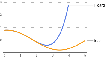
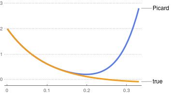
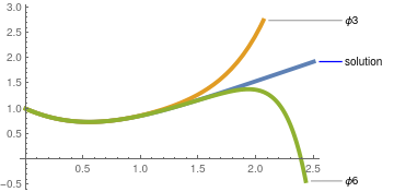
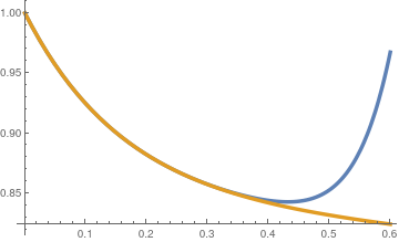
Note that Picard's iteration applied to the given second order differential equation (6.1) provides a better and more accurate approximation than approximation obtained from the first order system of equations (6.4). However, all these Picard's approximation contain noise terms caused by the differential equation with variable coefficients. Recall that Picard's approximations applied to autonomous equations do not contain noise terms and provide direct approximations to the true solution.
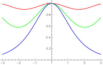
      Now we plot the true solution along with third and sixth Picard's approximations.
sol[t_] = E^-t^2 (1 - E^t^2 t + E^t^2 Sqrt[\[Pi]] t Erf[t]);
phi3[x_] = 1 - x + 2 (x^2/2 - x^4/12 + x^6/60);
phi6[x_] = 1 - x + 2 (x^2/2 - x^4/12 + x^6/60 - x^8/336 + x^10/2160 - x^12/ 15840);
Plot[{Callout[sol[x], "solution", CalloutStyle -> {Blue}], Callout[phi3[x], "\[Phi]3"], Callout[phi6[x], "\[Phi]6"]}, {x, 0, 2.5}, PlotStyle -> Thickness[0.014]]
       True solution and its third and sixth Picard approximations.            Mathematica code
   ■

Example 7: . Consider the initial value problem for the homogeneous Duffing equation:

\[ \ddot{y} + 2\eta\,\dot{y} + y + \varepsilon \, y^3 = 0 , \qquad y(0) = d, \quad \dot{y} (0) = v , \tag{7.1} \]
where d = 1 is the initial displacement and v =-1 is the initial velocity. For simplicity, we choose the following numerical values of parameters: η = 3 and ε = 1. First, we convert the given problem to a system of first order differential equations
\[ \frac{\text d}{{\text d}t} \begin{bmatrix} y_1 (t) \\ y_2 (t) \end{bmatrix} = \begin{bmatrix} y_2 \\ -2\eta\, y_2 - y_1 - \varepsilon\, y_1^3 \end{bmatrix} = \begin{bmatrix} y_2 \\ -6\, y_2 - y_1 - y_1^3 \end{bmatrix} , \qquad \begin{bmatrix} y_1 (0) \\ y_2 (0) \end{bmatrix} = \begin{bmatrix} \phantom{-}1 \\ -1 \end{bmatrix} . \tag{7.2} \]
Upon integration, we transfer this initial value problem into the Volterra integral equation:
\[ \begin{bmatrix} y_1 (t) \\ y_2 (t) \end{bmatrix} = \begin{bmatrix} \phantom{-}1 \\ -1 \end{bmatrix} + \int_0^t \begin{bmatrix} y_2 (s) \\ -6\, y_2 (s) - y_1 (s) - y_1^3 (s) \end{bmatrix} {\text d}s . \tag{7.3} \]
This allows us to set up the Picard iteration scheme explicitly:
\[ {\bf \phi}_0 = \begin{bmatrix} d \\ v \end{bmatrix} = \begin{bmatrix} \phantom{-}1 \\ -1 \end{bmatrix} , \qquad {\bf \phi}_{n+1} (t) = \begin{bmatrix} x_{n+1} (t) \\ y_{n+1} (t) \end{bmatrix} = \begin{bmatrix} d\\ v \end{bmatrix} + \int_0^t \, \begin{bmatrix} y_n (s) \\ - x_n (s) - \varepsilon\, x^3_n (s) - 2\eta\, y_n (s) \end{bmatrix}_n \, {\text d} s , \qquad n=0,1,2,\ldots . \tag{7.4} \]
We show each iteration separately.
\begin{align*} {\bf \phi}_1 &= \begin{bmatrix} \phantom{-}1 \\ -1 \end{bmatrix} + \int_0^t \, \begin{bmatrix} -1 \\ 6-1-1 \end{bmatrix} \, {\text d} s = \begin{bmatrix} 1-t \\ 4t-1 \end{bmatrix} , \\ {\bf \phi}_2 &= \begin{bmatrix} \phantom{-}1 \\ -1 \end{bmatrix} + \int_0^t \, \begin{bmatrix} 4s-1 \\ 6(1-4s) -(1-s) - (1-s)^3 \end{bmatrix} \, {\text d} s \\ &= \begin{bmatrix} \phantom{-}1 \\ -1 \end{bmatrix} + \int_0^t \begin{bmatrix} 4s-1 \\ \left[ 4 -20s -3 s^2 + s^3 \right] \end{bmatrix} \, {\text d} s = \begin{bmatrix} 1-t + 2t^2 \\ -1+ 4t - 10 t^2 - t^3 + \frac{t^4}{4} \end{bmatrix} , \\ {\bf \phi}_3 &= \begin{bmatrix} \phantom{-}1 \\ -1 \end{bmatrix} + \int_0^t \, \begin{bmatrix} -1+ 4s - 10 s^2 - s^3 + \frac{s^4}{4} \\ - \left( 1-s + 2s^2 \right) - \left( 1-s + 2s^2 \right)^3 - 6 \left( -1+ 4s - 10 s^2 - s^3 + \frac{s^4}{4} \right) \end{bmatrix} \, {\text d} s \\ &= \begin{bmatrix} 1-t + 2t^2 - \frac{10}{3}\, t^3 - \frac{t^4}{4} + \frac{t^5}{20} \\ -1 + 4t - 10 t^2 + \frac{49}{3}\, t^3 + \frac{19}{4}\, t^4 - \frac{39}{10}\, t^5 + 2\,t^6 - \frac{8}{7} \, t^7 \end{bmatrix} , \\ {\bf \phi}_4 &= \begin{bmatrix} 1 \\ -1 \end{bmatrix} + \int_0^t \, \begin{bmatrix} -1 + 4s - 10 s^2 + \frac{49}{3}\, s^3 + \frac{19}{4}\, s^4 - \frac{39}{10}\, s^5 + 2\,s^6 - \frac{8}{7} \, s^7 \\ 4- 20t + \cdots \end{bmatrix} {\text d} s \\ &= \begin{bmatrix} 1-t + 2t^2 - \frac{10}{3}\, t^3 + \frac{49}{12}\, t^4 + \frac{19}{20}\, t^5 - \frac{13}{20}\, t^6 + \frac{2}{7}\, t^7 - \frac{1}{7}\, t^8 \\ -1 + 4t - 10 t^2 + \frac{49}{3}\, t^3 - \frac{215}{12}\, t^4 - \frac{131}{10}\, t^5 + \frac{279}{20}\, t^6 - \frac{5357}{420} \, t^7 + \cdots \end{bmatrix} . \end{align*}
Of course, all these manipulations we delegate to Mathematica. To check the quality of Picard's iteration scheme, we compare the expansions obtained with correct Maclaurin expansion:
AsymptoticDSolveValue[{y''[t] + 6*y'[t] + y[t] -(y[t])^3 == 0, y[0] == 1, y'[0] == -1}, y[t], {t, 0, 10}]
-t + 3 t^2 - (19 t^3)/3 + (41 t^4)/4 - (833 t^5)/60 + (511 t^6)/30 - ( 12937 t^7)/630 + (17477 t^8)/672 - (3211123 t^9)/90720 + ( 306715 t^10)/6048
\[ y(t) = 1-t + 3\,t^2 - \frac{19}{3}\,t^3 + \frac{41}{4}\, t^4 - \frac{833}{60}\,t^5 + \frac{511}{30}\,t^6 - \frac{12937}{630}\,t^7 + \cdots . \]
     
sol = NDSolve[{y''[t] + 6*y'[t] + y[t] - (y[t])^3 == 0, y[0] == 1, y'[0] == -1}, y[t], {t, 0, 10}];
AsymptoticDSolveValue[{y''[t] + 6*y'[t] + y[t] - (y[t])^3 == 0, y[0] == 1, y'[0] == -1}, y[t], {t, 0, 10}]
pol[t_] = 1 - t + 3 t^2 - (19 t^3)/3 + (41 t^4)/4 - (833 t^5)/60 + (511 t^6)/ 30 - (12937 t^7)/630 + (17477 t^8)/672 - (3211123 t^9)/90720 + ( 306715 t^10)/6048;
Plot[{pol[t], Evaluate[y[t] /. sol]}, {t, 0, 0.6}, PlotStyle -> Thick
       True solution of Duffing's equation and its 10-term approximation (in blue).            Mathematica code
   ■

Example 8: Jacobi Elliptic functions.

Carl Jacobi.

The German mathematician Carl Gustav Jakob Jacobi (1804--1851) came from a Jewish family but he was given the French style name Jacques Simon at birth. His father, Simon Jacobi, was a banker and his family was prosperous. Carl was the second son of the family, the eldest being Moritz Jacobi who eventually became a famous physicist. In 1825 Carl obtained the degree of Doctor of Philosophy with a dissertation on the partial fraction decomposition of rational fractions defended before a commission led by Enno Dirksen. He followed immediately with his Habilitation and at the same time converted to Christianity. Now qualifying for teaching University classes, the 21-year-old Jacobi lectured in 1825/26 on the theory of curves and surfaces at the University of Berlin (Prussia).

In 1827 he became a professor and in 1829, a tenured professor of mathematics at Königsberg University, and held the chair until 1842. Jacobi was the first Jewish mathematician to be appointed professor at a German university. Jacobi suffered a breakdown from overwork in 1843. He then visited Italy for a few months to regain his health. On his return he moved to Berlin, where he lived as a royal pensioner until his death. One of Jacobi's greatest accomplishments was his theory of elliptic functions and their relation to the elliptic theta function.

Consider the initial value problem

\[ \dot{x} ( t ) = y\, z, \quad \dot{y} (t) = -x\,z, \quad \dot{z} (t) = -k^2 x\,y , \qquad x(0) =0, \quad y(0) =1, \quad z(0) =1, \tag{8.1} \]
where dots stand for derivatives with respect to t, and k denotes a positive constant \( \le 1 . \) The parameter k is known as the modulus; its complementary modulus is \( \kappa = \sqrt{1-k^2} . \) The solutions to the initial value problem above are usually called the basic Jacobi elliptic functions and denoted as
\[ x(t) = \mbox{sn} (t) , \qquad y(t) = \mbox{cn}(t) , \qquad z(t) = \mbox{dn} (t) . \]

These functions were introduced by Jacobi in 1829. They are found in the description of the motion of a pendulum (see also pendulum (mathematics)), as well as in the design of the electronic elliptic filters.

Using Picard's iteration we derive the sequence

\begin{eqnarray*} \tag{8.2} x_{(k+1)} (t) &=& \int_0^t y_{(k)} (s)\,z_{(k)} (s) \,{\text d}s , \\ y_{(k+1)} (t) &=& 1 - \int_0^t x_{(k)} (s)\,z_{(k)} (s) \,{\text d}s , \\ z_{(k+1)} (t) &=& 1 - k^2 \int_0^t x_{(k)} (s)\,y_{(k)} (s) \,{\text d}s , \end{eqnarray*}
where initially x0 = 0, y0 = 1, z0 = 1. The first iteration becomes
\begin{eqnarray*} x_{(1)} (t) &=& \int_0^t y_{(0)} (s)\,z_{(0)} (s) \,{\text d}s = \int_0^t \,{\text d}s = t , \\ y_{(1)} (t) &=& 1 - \int_0^t x_{(0)} (s)\,z_{(0)} (s) \,{\text d}s =1, \\ z_{(1)} (t) &=& 1 - k^2 \int_0^t x_{(0)} (s)\,y_{(0)} (s) \,{\text d}s = 1 \end{eqnarray*}
because x0 = 0 and y0 = z0 = 1.

Second iteration is

\begin{eqnarray*} x_{(2)} (t) &=& \int_0^t y_{(1)} (s)\,z_{(1)} (s) \,{\text d}s = \int_0^t \,{\text d}s = t , \\ y_{(2)} (t) &=& 1 - \int_0^t x_{(1)} (s)\,z_{(1)} (s) \,{\text d}s =1- \int_0^t s\, {\text d}s = 1 - \frac{t^2}{2} , \\ z_{(2)} (t) &=& 1 - k^2 \int_0^t x_{(1)} (s)\,y_{(1)} (s) \,{\text d}s = 1 - k^2 \int_0^t s\, {\text d}s = 1 - k^2 \frac{t^2}{2} . \end{eqnarray*}
If we proceed successively, we find that the coefficients of the various powers of t ultimately become stable, i.e., they remain unchanged in successive iterations. This leads to the representation of solutions as convergent power series, which are usually denoted by the symbols snt (or sn(t.m) for m=k2), cnt, and dnt, and are called sine amplitude, cosine amplitude, and delta amplitude, respectively. These functions were introduced by Carl Jacobi in 1829.
\begin{eqnarray*} \mbox{sn} (t,k) &=& t - \left( 1 + k^2 \right) \frac{t^3}{3!} + \left( 1 + 14 k^2 + k^4 \right) \frac{t^5}{5!} - \left( 1 + 135 k^2 + 135 t^4 + k^6 \right) \frac{t^7}{7!} + O\left( t^9 \right) , \\ \mbox{cn} (t,k) &=& 1 - \frac{t^2}{2!} + \left( 1+ 4k^2 \right) \frac{t^4}{4!} - \left( 1 + 44k^2 + 16 k^4 \right) \frac{t^6}{6!} + O\left( t^8 \right) , \\ \mbox{dn} (t,k) &=& 1 - k^2 \frac{t^2}{2!} + k^2 \left( 4 + k^2 \right) \frac{t^4}{4!} - k^2 \left( 16 + 44k^2 + k^4 \right) \frac{t^6}{6!} + O\left( t^8 \right) . \end{eqnarray*}

Each of Jacobi elliptic functions satisfy a single-variable equation:

  • sn(t) solves the differential equations
    \[ \frac{{\text d}^2 y}{{\text d}t^2} + \left( 1 + k^2 \right) y - 2\,k^2 y^3 =0 \qquad\mbox{and} \qquad \left( \frac{{\text d} y}{{\text d}t} \right)^2 = \left( 1- y^2 \right) \left( 1 - k^2 y^2 \right) . \]
  • cn(t) solves the differential equations
    \[ \frac{{\text d}^2 y}{{\text d}t^2} + \left( 1 -2\, k^2 \right) y + 2\,k^2 y^3 =0 \qquad\mbox{and} \qquad \left( \frac{{\text d} y}{{\text d}t} \right)^2 = \left( 1- y^2 \right) \left( 1 - k^2 + k^2 y^2 \right) . \]
  • dn(t) solves the differential equations
    \[ \frac{{\text d}^2 y}{{\text d}t^2} - \left( 2 - k^2 \right) y + 2\, y^3 =0 \qquad\mbox{and} \qquad \left( \frac{{\text d} y}{{\text d}t} \right)^2 = \left( y^2 -1 \right) \left( 1 - k^2 - y^2 \right) . \]
The functions satisfy the two square relations
\begin{eqnarray*} \mbox{cn}^2 (t) + \mbox{sn}^2 (t) &=& 1 , \\ \mbox{dn}^2 (t) + k^2 \mbox{sn}^2 (t) &=& 1 . \end{eqnarray*}
These functions are doubly periodic generalizations of the trigonometric functions satisfying
\begin{eqnarray*} \mbox{sn} (t,0) &=& \sin t , \\ \mbox{cn} (t,0) &=& \cos t , \\ \mbox{dn} (t,0) &=& 1 . \end{eqnarray*}
Now we plot some of them:
Plot[Tooltip@{JacobiSN[x, 1/5], JacobiSN[x, 2/3], JacobiSN[x, 1]}, {x, -3, 3},
PlotStyle -> {Red, Green, Blue}] /. {Tooltip[{_, color_, line_}, tip_] :> {Text[Style[tip, 14], {.1, 0} + line[[1, -1]]], color, line}}
Plot[Tooltip@{JacobiCN[x, 1/5], JacobiCN[x, 2/3], JacobiCN[x, 1]}, {x, -3, 3},
PlotStyle -> {Red, Green, Blue}] /. {Tooltip[{_, color_, line_}, tip_] :> {Text[Style[tip, 14], {.1, 0} + line[[1, -1]]], color, line}}
Plot[Tooltip@{JacobiDN[x, 1/5], JacobiDN[x, 2/3], JacobiDN[x, 1]}, {x, -3, 3},
PlotStyle -> {Red, Green, Blue}] /. {Tooltip[{_, color_, line_}, tip_] :> {Text[Style[tip, 14], {.1, 0} + line[[1, -1]]], color, line}}


       graphs of sn(x,k)        graphs of cn(x,k)        graphs of dn(x,k)
   ■


  1. Djang, G.-F., A modified method of iteration of the Picard type in the solution of differential equations, Journal of The Franklin Institute, 1948, Vol. 246, Issue 6, pp. 453--457. https://doi.org/10.1016/0016-0032(48)90261-0
  2. Fabrey, J., Picard's theorem, The American Mathematical Monthly, 1972,Vol. 79, No. 9, pp. 1020--1023
  3. Hu, J. and Li, W.-P., Theory of Ordinary Differential Equations, The Hong Kong University of Science and Technology, 2005.
  4. Let's Learn, Nemo, YouTube.
  5. Robin, W.A., Solving differential equations using modified Picard iteration, International Journal of Mathematical Education in Science and Technology, Volume 41, 2010, Issue 5, Pages 649--665; https://doi.org/10.1080/00207391003675182


Return to Mathematica page
Return to the main page (APMA0340)
Return to the Part 1 Matrix Algebra
Return to the Part 2 Linear Systems of Ordinary Differential Equations
Return to the Part 3 Non-linear Systems of Ordinary Differential Equations
Return to the Part 4 Numerical Methods
Return to the Part 5 Fourier Series
Return to the Part 6 Partial Differential Equations
Return to the Part 7 Special Functions