Preface
This section gives an introduction to two dimensional (also called planar) systems of ordinary differential equations.
Return to computing page for the first course APMA0330
Return to computing page for the second course APMA0340
Return to Mathematica tutorial for the first course APMA0330
Return to Mathematica tutorial for the second course APMA0340
Return to the main page for the first course APMA0330
Return to the main page for the second course APMA0340
Return to Part III of the course APMA0340
Introduction to Linear Algebra with Mathematica
Glossary
Planar equations
A tangent vector at each given point can be calculated directly from the given matrix-vector equation \( \dot{\bf x} = {\bf A}\,{\bf Ax} , \) using the position vector x = (x1, x2).
In first part of the course, we discussed the direction field for first order differential equations. The construction of a direction field is equally useful in the study of autonomous systems (when slope vector does not depend on time explicitly) of two first-order equations. It provides an overall view of where the solution curves go, and the arrows show which way the system moves as time increases.
A phase portrait of a planar system is a representative set of its solutions, plotted as parametric curves (with t as the parameter) on the Cartesian plane tracing the path of each particular solution (x, y) = (x1(t), x2(t)), −∞ < t < ∞. Similar to a direction field, a phase portrait is a graphical tool to visualize how the solutions of a given system of differential equations would behave in the long run. Just like a direction field, a phase portrait can be a tool to predict the behaviors of a system’s solutions. To do so, we draw a grid on the phase plane. Then, at each grid point x = (α, β), we can calculate the solution trajectory’s instantaneous direction of motion at that point by using the given system of equations to compute the tangent / velocity vector, x′ In this context, the Cartesian plane where the phase portrait resides is called the phase plane. The parametric curves traced by the solutions are sometimes also called their trajectories.
Mathematica utilizes several dedicated commands for plotting phase portraits: VectorPlot and ListVectorPlot3D, VectorDensityPlot, SliceVectorPlot3D, and StreamPlot, StreamDensityPlot, ListStreamPlot, LineIntegralConvolutionPlot; they may include ParametricPlot, DensityPlot for plotting such direction fields.
We consider systems of first order ordinary differential equations in normal form on the planeIf an initial position of the vector \( {\bf x} (t) \) is known, we get an initial value problem:
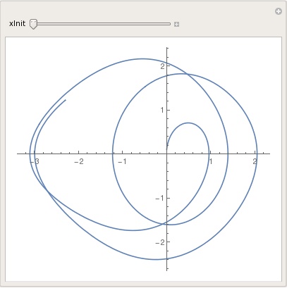
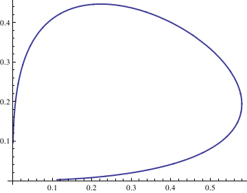
It is convenient to use Manipulate command to analyze dependence of solutions on some input parameters. First, we demonstrate dependence of solution of the damped pendulum equation with periodic input
\( x'' + 0.1\, x' + \sin (x) = \cos t, \quad x(0) =a, \ x' (0) =0.1 \)
on the input initial position.
|
Manipulate[
sol = NDSolve[{x''[t] + 0.1*x'[t] + Sin[x[t]] == Cos[t], x[0] == xInit, x'[0] == 0.1}, {x}, {t, 0, 50}]; ParametricPlot[Evaluate[{x[t], x'[t]} /. sol, {t, 0, 20}]], {xInit, 0, 1}] Export["pendulum4.png", %] |
|
| Plot of solution to driven pendulum equation. | Mathematica code |
For autonomous systems with two dimensional phase space, three types of trajectories are possible. A trajectory consisting of single point (corresponding to equilibrium solutions), and if trajectory has more than one point, then it could be a closed curve (corresponding to periodic solutions), or a curve without self-intersection. For autonomous systems in three or more dimensions, there could be other kinds of trajectories, including chaotic orbits (see next chapter).
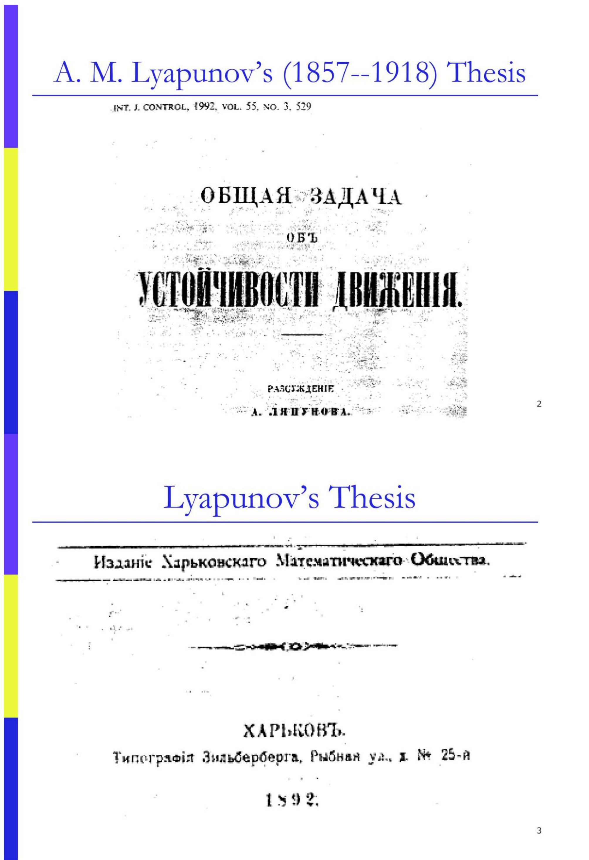
There are several definitions of stability of critical points for systems of first order differential equations. Historically, the first rigorous definition of stability using ε-δ-notation was proposed in 1892 by the Russian mathematician A.M. Lyapunov (1857--1918).
-
Stable (in the sense of Lyapunov) when, given arbitrary ε > 0, there exists a δ = δ(ε) > 0 so small that if
\begin{equation} \label{EqStable.1a} \left\vert x(0) - a \right\vert < \delta , \qquad \left\vert y(0) - b \right\vert < \delta , \end{equation}then\begin{equation} \label{EqStable.2a} \left\vert x(t) - a \right\vert < \varepsilon , \qquad \left\vert y(t) - b \right\vert < \varepsilon , \end{equation}for all t > 0 and all orbits x = x(t), y = y(t) of the system \eqref{EqPlanar.1}.
-
Asymptotically stable if it is Lyapunov stable and there exists δ > 0 such that relations \eqref{EqStable.1a} imply
\begin{equation} \label{EqStable.3a} \lim_{t\to\infty} \left\vert x(t) - a \right\vert =0 , \qquad \lim_{t\to\infty} \left\vert y(t) - b \right\vert =0 , \end{equation}for all trajectories of x = x(t), y = y(t) of the system \eqref{EqPlanar.1}.
-
Uniformly stable if, for each ε > 0 there is a δ = δ(ε) > 0 independent of the initial t0 such that
\[ |x\left( t_0 \right) | < \delta , \quad |y\left( t_0 \right) | < \delta , \quad \Longrightarrow \quad |x(t) < \varepsilon , \ |y(t) < \varepsilon , \qquad \forall t \ge t_0 \ge 0, \]is satisfied, for all t0 ≥ 0.
- Unstable when it is not stable.
Critical Points of Planar Autonomous Systems
This sounds like a good idea, but there is a problem with it: How can we be assured that the nonlinear terms that we have truncated do not play a significant role in determining the local behavior? The answer to this question is provided by famous Grobman--Hartman theorem., discussed in section.
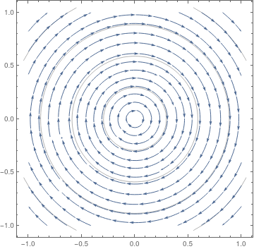
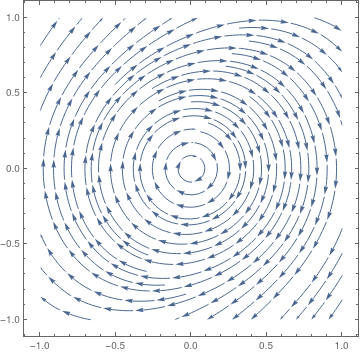
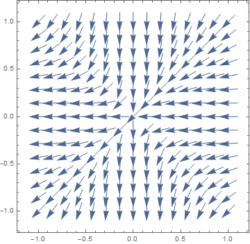
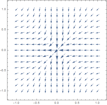
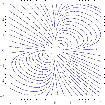
As an example of the sort of thing that can go wrong, consider a standard harmonic oscillator and its nonlinear perturbation:
|
|
|
| Linear oscilaltor (stable). | Nonlinear oscillator (unstable). |
StreamPlot[{y, 0.5*y^3 - x}, {x, -1, 1}, {y, -1, 1}, StreamScale -> {{0.1, 0.1}, Automatic}]
In order to use the linear equations for characterization of an equilibrium point of nonlinear system, we need sufficient conditions that guarantee the use of linearization. Since a linear system is completely characterized by its eigenvalues, we need sufficient conditions for a relation between the Jacobian and the corresponding nonlinear system.
2. An equilibrium point in a nonlinear system is Lyapunov unstable if there exists at least one eigenvalue of the corresponding Jacobian that has a positive real part.
Thus, Lyapunov’s theorems state that if the equilibrium is hyperbolic, then the linearized system of equations correctly predict the Lyapunov stability in the nonlinear system. (Note that in the second of Lyapunov’s theorems, it is not necessary for the equilibrium to be hyperbolic since the presence of an eigenvalue with positive real part implies instability even if it is accompanied by other eigenvalues with zero real part.) If an equilibrium point is hyperbolic, then we saw that the linear system of equations correctlyrepresent the nonlinear system locally, as far as Lyapunov stability goes. For a hyperbolic equilibrium point, the topology of the linearized system is the same as the topology of the nonlinear system in some neighborhood of the equilibrium point. Specifically, for a hyperbolic equilibrium point P, there is a continuous 1:1 invertible transformation (a homeomorphism) defined on some neighborhood of P that maps the motions of the nonlinear system to the motions of the linearized system. This is called the Grobman--Hartman theorem
To clasify isolated equilibria, it is convenient to employ polar coordinates cenetred at the critical point: r = ρ(t), θ = ω(t). Recall that there are four types of critical points:-
Nodes are critical points with the property that a trajectories arrive or depart from the critical point along some directory. In turn, there are know of three types of nodes:
- proper node or star (when every semiline from the critical point is a tangent to some orbit);
- improper node when there are at most two directions along which trajectories approach the critical point;
- degenerate node when there is only one direction along which orbits approach the critical point.
- Saddle points.
- Centers (or vortex) when trajectories travel in closed elliptical orbits in some direction around the critical point.
- Spirals (when written in polar coordinates r = ρ(t), θ = ω(t), these functions sutisfy \( \lim_{t\to +\infty} |\omega (t)| = 0 \quad\mbox{or}\quad \lim_{t\to -\infty} |\omega (t)| = 0 \) in some neighbohood of the critical point).
| eigenvalues | linear system | nonlinear system | ||||
|---|---|---|---|---|---|---|
| real | both positive | equal | proper or improper node | unstable | similar to node or spiral point | unstable |
| different | node | unstable | same | |||
| both negative | equal | proper or improper node | as. stable | similar to node or spiral point | as. stable | |
| different | node | as. stable | same | |||
| positive and negative | saddle point | unstable | same | |||
| complex not real |
real part positive. | spiral point | unstable | same | ||
| real part negative | spiral point | as. stable | same | |||
| real part zero | center | stable | similar to center or spiral point | ? | ||
``same'' means that type and stability for the nonlinear problem are the same as for the corresponding linear problem. If we look at at smaller and smaller neighborhoods of the critical point, the phase portrait looks more and more like the phase portrait of the corresponding linear system.
``?'' means that this cannot be determined on basis of the corresponding linear problem.
Note that the table only considers the case of nonzero eigenvalues. In this case we always have an isolated critical point.
Some Examples of Planar Systems
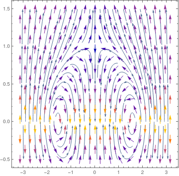
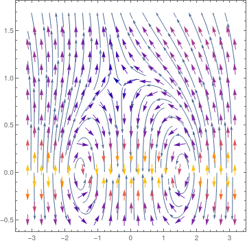
We plot phase portrates for two cases, when grad force is taking into account and when it is neglected.
p = StreamPlot[{-Sin[u], (v^2 - Cos[u])/v}, {u, -Pi, Pi}, {v, -0.5, 1.5}, MaxRecursion -> 5];
Show[sp, vp] sp2 = StreamPlot[{-Sin[u] - 0.5*v^2, (v^2 - Cos[u])/v}, {u, -Pi, Pi}, {v, -0.5, 1.7}, MaxRecursion -> 5];
vp2 = VectorPlot[{-Sin[u] - 0.5*v^2, (v^2 - Cos[u])/v}, {u, -Pi, Pi}, {v, -0.5, 1.5}, MaxRecursion -> 5];
Show[sp2, vp2]
|
|
|
| Phase portrait without drag force. | Phase portrait with drag force. |
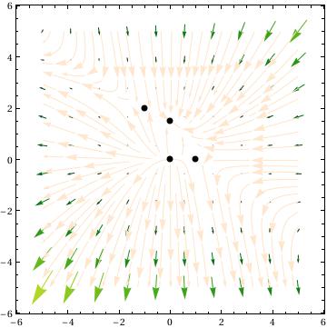
Consider the following non-linear system of ordinary differential equations
ydot1[x_, y_] := 3 y - x*y - 2 y^2;
a = Solve[{xdot1[x, y] == 0, ydot1[x, y] == 0}, {x, y}, Reals]
b = Reap[Do[Sow[{x, y} /. i], {i, a}]][[2, 1]]
Reap[Do[Sow[Eigenvalues[mat1[x, y] /. a[[n]]]], {n, Length[a]}]][[2, 1]]
mat1[x_, y_] = {{D[xdot1[x, y], x],
D[xdot1[x, y], y]}, {D[ydot1[x, y], x], D[ydot1[x, y], y]}}
Out[4]= {{-1, 2}, {0, 0}, {0, 3/2}, {1, 0}}
Out[5]=
{Eigenvalues[mat1[-1, 2]], Eigenvalues[mat1[0, 0]],
Eigenvalues[mat1[0, 3/2]], Eigenvalues[mat1[1, 0]]}
Out[6]= {{1 - 2 x - y, -x}, {-y, 3 - x - 4 y}}
Eigenvalues[c]
d = mat1[b[[2, 1]], b[[2, 2]]]
Eigenvalues[d]
Out[8]= {1/2 (-3 - Sqrt[17]), 1/2 (-3 + Sqrt[17])}
Out[9]= {{1, 0}, {0, 3}}
Out[10]= {3, 1}
Eigenvalues[e]
f = mat1[b[[4, 1]], b[[4, 2]]]
Eigenvalues[f]
Out[12]= {-3, -(1/2)}
Out[13]= {{-1, -1}, {0, 2}}
Out[14]= {2, -1}
StreamScale -> Large, StreamStyle -> LightOrange, VectorPoints -> 10,
VectorColorFunction -> "AvocadoColors", Epilog -> {PointSize[Large], Point[b]}]
Out[23]= {{x -> -1, y -> 2}, {x -> 0, y -> 0}, {x -> 0, y -> 3/2}, {x -> 1, y -> 0}}
Out[24]= {{-1, 2}, {0, 0}, {0, 3/2}, {1, 0}}
Out[25]= {Eigenvalues[mat1[-1, 2]], Eigenvalues[mat1[0, 0]],
Eigenvalues[mat1[0, 3/2]], Eigenvalues[mat1[1, 0]]}
Out[26]= {{1 - 2 x - y, -x}, {-y, 3 - x - 4 y}}
Out[27]= {{1, 1}, {-2, -4}}
Out[28]= {1/2 (-3 - Sqrt[17]), 1/2 (-3 + Sqrt[17])}
Out[29]= {{1, 0}, {0, 3}}
Out[30]= {3, 1}
Out[31]= {{-(1/2), 0}, {-(3/2), -3}}
Out[32]= {-3, -(1/2)}
Out[33]= {{-1, -1}, {0, 2}}
Out[34]= {2, -1}
Explanation:
This command solves for all of the critical points and stores them as "a"
This command transforms the critical points so that they are no longer in a list with x's and y's. This allows you to plot all of the critical points.
This command creates a function of the matrix used for linearization.
This command create a list of matrices, where each matrix corresponds to one of the critical points from the list in "a". Order is preserved so the first critical point will be associated with the first matrix in c.
This command creates a list of eigenvalues, where each set of eigenvalues corresponds to one of the critical points. Order is preserved so the first critical point will be associated with the the first set of eigenvalues.
The plot, which uses "b" to plot all of the critical point. "a" cannot be used here because it is not of the correct form for the function epilog which plots points.
StreamScale -> Large, StreamStyle -> LightOrange, VectorPoints -> 10,
VectorColorFunction -> "AvocadoColors", Epilog -> {PointSize[Large], Point[b]}]
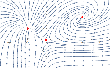
Example 2. We can plot the phase portrait manually:
pp = ListPlot[{{0, 0}, {-2, 2}, {4, 4}}, PlotStyle -> {Thick, Red, PointSize[Large]}, PlotRange -> {{-5, 7}, {-5, 7}}]
Show[pp, sp]
{y, -1, 1}, VectorScale -> {Automatic, Automatic, #}] & /@ {None, Function[If[#5 > 50, None, #5^.3]]}
 |
 |
f2[x_, y_] = Simplify[D[f[x, y], y]]
f1[x_, y_] = Simplify[D[f[x, y], x]]
Show[ContourPlot[f[x, y], {x, -1, 1}, {y, -1, 1}, ContourStyle -> Directive[Red, Dashed],
ColorFunction -> "Rainbow", Contours -> 20],
VectorPlot[{f1[x, y], f2[x, y]}, {x, -1, 1}, {y, -1, 1},
VectorScale -> {Automatic, Automatic, Function[If[#5 > 50, None, #5^.3]]}, VectorStyle -> Black]]
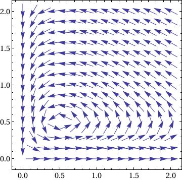
2.3.2. Autonomous Systems
Print["X' = ", MatrixForm[f[x, y]]]
X' = (x-2 x y
-0.5 y+x y )
x' = x-2 x y, y' = -0.5 y+x y
BaseStyle -> {FontFamily -> "Times", FontSize -> 14}]
f[x, y]/(10^-8 + Norm[f[x, y]]), {x, 0, 2}, {y, 0, 2}],
Frame -> True, BaseStyle -> {FontFamily -> "Times", FontSize -> 14}]
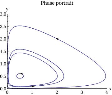
ParametricPlot[
Table[{x[t], y[t]} /. sol[[j]], {j, Length[ic]}], {t, 0, T},
PlotRange -> {{0, 4}, {0, 3}}],
Table[Graphics[{Arrowheads[.03],
Arrow[{ic[[j]], ic[[j]] + .01 f[ic[[j, 1]], ic[[j, 2]] ] }]}],
{j, Length[ic]}],
AxesLabel -> {"x", "y"},
BaseStyle -> {FontFamily -> "Times", FontSize -> 14},
PlotLabel -> "Phase portrait"
]
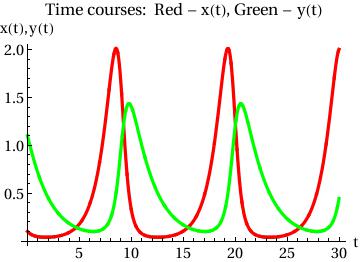
PlotStyle -> {{Thickness[0.01], RGBColor[1, 0, 0]}, {Thickness[0.01],
RGBColor[0, 1, 0]}}, AxesOrigin -> {0, 0},
AxesLabel -> {"t", "x(t),y(t)"},
BaseStyle -> {FontFamily -> "Times", FontSize -> 14},
PlotLabel -> "Time courses: Red - x(t), Green - y(t)"]
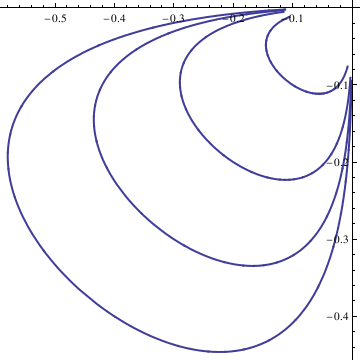
Example. Consider the system of autonomous equations
deq2 = y'[t] == 2*x[t]*y[t] - y[t]^2;
soln = NDSolve[{deq1, deq2, x[0] == 1, y[0] == 1}, {x[t], y[t]}, {t, -10, 10}];
Do[Clear[x, y];
soln = NDSolve[{deq1, deq2, x[0] == n/10, y[0] == n/10}, {x[t], y[t]}, {t, -10, 10}];
x = soln[[1, 1, 2]];
y = soln[[1, 2, 2]];
curve[[n]] = ParametricPlot[{x, y}, {t, -10, 10}, PlotStyle -> Thick], {n, -4, 4}];
Show[curve[[-4]], curve[[-3]], curve[[-2]], curve[[-1]], curve[[1]], curve[[2]], curve[[3]], curve[[4]], AspectRatio -> 1]
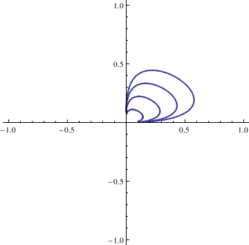
soln = NDSolve[{deq1, deq2, x[0] == n/10, y[0] == n/10}, {x[t], y[t]}, {t, -10, 10}];
x = soln[[1, 1, 2]];
y = soln[[1, 2, 2]];
curvep[[n]] = ParametricPlot[{x, y}, {t, -10, 10}, PlotStyle -> Thick], {n, 0, 4}];
Show[curvep[[0]], curvep[[1]], curvep[[2]], curvep[[3]], curvep[[4]], AspectRatio -> 1]
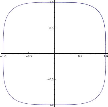
G[x_, y_] := x^3;
sol = NDSolve[{x'[t] == F[x[t], y[t]], y'[t] == G[x[t], y[t]],
x[0] == 1, y[0] == 0}, {x, y}, {t, 0, 3*Pi},
WorkingPrecision -> 20]
ParametricPlot[Evaluate[{x[t], y[t]}] /. sol, {t, 0, 3*Pi}]
Y[t_] := Evaluate[y[t] /. sol]
fns[t_] := {X[t], Y[t]};
len := Length[fns[t]];
Plot[Evaluate[fns[t]], {t, 0, 3*Pi}]
Applications
G[x_, y_] := x^3;
sol = NDSolve[{x'[t] == F[x[t], y[t]], y'[t] == G[x[t], y[t]],
x[0] == 1, y[0] == 0}, {x, y}, {t, 0, 3*Pi},
WorkingPrecision -> 20]
ParametricPlot[Evaluate[{x[t], y[t]}] /. sol, {t, 0, 3*Pi}]
{{x -> InterpolatingFunction[{{0, 9.4247779607693797154}}, <>],
y -> InterpolatingFunction[{{0, 9.4247779607693797154}}, <>]}}
Y[t_] := Evaluate[y[t] /. sol]
fns[t_] := {X[t], Y[t]};
len := Length[fns[t]];
Plot[Evaluate[fns[t]], {t, 0, 3*Pi}]
Return to Mathematica page
Return to the main page (APMA0340)
Return to the Part 1 Matrix Algebra
Return to the Part 2 Linear Systems of Ordinary Differential Equations
Return to the Part 3 Non-linear Systems of Ordinary Differential Equations
Return to the Part 4 Numerical Methods
Return to the Part 5 Fourier Series
Return to the Part 6 Partial Differential Equations
Return to the Part 7 Special Functions