Return to computing page for the first course APMA0330
Return to computing page for the second course APMA0340
Return to Mathematica tutorial for the first course APMA0330
Return to Mathematica tutorial for the second course APMA0340
Return to the main page for the first course APMA0330
Return to the main page for the second course APMA0340
Return to Part V of the course APMA0340
Introduction to Linear Algebra with Mathematica

Preface


Since a Fourier series may fail to converge at individual points, we are led to try to overcome this failure by interpreting the limit of partial sums in a different sense. This section presents an introduction to Cesàro summation and its application to Fourier series. Cesàro summation is one of possible regularizations of series with alternating coefficients---their numerical evaluations usually lead to an ill-posed problem.

Cesàro summation


Ernesto Cesàro

Fourier series allow us to represent a rather complicated function defined on a finite interval as a linear combination (which is usually infinite) of its projections onto a basis that consists of trigonometric functions. Such a compact representation has proven exceedingly useful in the analysis of many real-world systems involving periodic phenomena, such as waves propagating on a string, electrical circuits with oscillating current sources, and heat diffusion on a metal ring---an application we will later examine in detail. More generally, Fourier series usually arise in the ubiquitous context of boundary value problems, making them a fundamental tool among mathematicians, scientists, and engineers.

However, there lies a caveat. Except in degenerate cases, a Fourier series (more precisely, its finite sum truncation version,

\begin{equation} \label{EqCesaro.1} F_N (x) = \frac{a_0}{2} + \sum_{k=1}^N \left( a_k \cos \frac{k\pi x}{\ell} + b_k \sin \frac{k\pi x}{\ell} \right) = \sum_{k=-N}^N \alpha_k e^{k{\bf j} \pi x/\ell} , \end{equation}
with which we deal in applications) is usually not an exact replica of the original function. Thus, a natural question is: exactly how does the truncated sum \( F_N (x) \) approximate the function? If we say that the Fourier series converges to the function, then precisely in what sense does the series converge? And under what conditions on function f?

When dealing with orthogonal expansions, it is convenient to utilize notion of 𝔏²-convergence, or convergence in the square mean. We consider only functions defined on a finite interval of length 2ℓ. Once we represent this function as a Fourier series, we get its periodic extension with period T = 2ℓ. Therefore, it is convenient to assume that the original function is a periodic function. Then its convergent Fourier series gives exact equality for the given function. For a 2ℓ-periodic function f, we have 𝔏²-convergence of the Fourier series FN(x) if

\[ \lim_{N\to \infty} \,\int_{-\ell}^{\ell} \left\vert f(x) - F_N (x) \right\vert^2 {\text d} x = \lim_{N\to \infty} \,\int_{-\ell}^{\ell} \left\vert f(x) - \sum_{n=-N}^N \hat{f}(n)\, e^{n{\bf j} \pi x/\ell} \right\vert^2 {\text d} x = 0 , \]
where
\[ \hat{f}(n) = \frac{1}{2\ell} \int_{-\ell}^{\ell} f(x)\,e^{-n{\bf j} \pi x/\ell} {\text d} x , \qquad n= 0, \pm 1, \pm 2, \ldots . \]

One of the first results regarding Fourier series convergence is that if f is square-integrable (that is, if \( \int_{-\ell}^{\ell} \left\vert f(x) \right\vert^2 {\text d} x < \infty \) ), then its Fourier series 𝔏²-converges to f(x). This is a nice result, but it leaves more to be desired. 𝔏²-convergence only says that over an interval of length 2ℓ, the average deviation between f(x) and its Fourier approximation FN(x) must tend to zero. However, for a fixed x in \( (-\ell , \ell ) , \) there are no guarantees on the difference between f(x) and the series approximation at x.

A stronger---and quite natural---sense of convergence is pointwise convergence, in which we demand that at each point \( x \in (-\ell ,\ell ), \) the series approximation converges to f(x). The Pointwise Convergence Theorem then states that if f is sectionally continuous and x0 is such that the one-sided derivatives \( f' (x_0 +0) = \lim_{\epsilon \,\mapsto 0, \epsilon >0} \, f(x_0 +\epsilon ) \) and \( f' (x_0 -0) = \lim_{\epsilon\, \mapsto 0, \epsilon >0} \, f(x_0 -\epsilon ) \) both exist, then the Fourier series converges to \( f (x_0 ) . \) However, in cases when the function experiences a finite jump of discontinuity pointwise convergence is not an appropriate notion of convergence as Gibbs phenomenon shows.

To avoid such problems, we desire the even stronger notion of uniform convergence, such that the rate at which the series converges is identical for all points in \( [-\ell , \ell ] , \) and consequently, everywhere (due to periodicity). By adopting the metric

\[ d(f,g) = \| f(x)-g(x) \|_{\infty} = \sup_x \left\{ |f(x)-g(x)) \, : \, x\in [-\ell , \ell ] \right\} \]
over the space of continuous functions from \( [-\ell , \ell ] \) to \( \mathbb{R} , \) we can force convergence to imply uniform convergence, simply by definition. This metric space is denoted by \( C([-\ell , \ell ], \mathbb{R}) . \) It can also be proven that \( C([-\ell , \ell ], \mathbb{R}) \) is a vector space, and thus the concept of series is well-defined.

To define uniform convergence of Fourier series, we need a more general definition of convergence for infinite sum, that is known as 
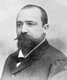
Cesàro summation, named after the Italian analyst Ernesto Cesàro (1859--1906). Recall the definition of Cesàro summability of infinite series (which is capable of finding sums of divergent series).

Let \( \{ a_k \} \) be a sequence, and let

\[ s_n = a_1 + a_2 + \cdots + a_n =\sum_{k=1}^n a_k \qquad \mbox{or} \qquad S_n = a_0 + a_1 + \cdots + a_n =\sum_{k=0}^n a_k \]
be the nth partial sum of the series
\[ \sum_{k=1}^{\infty} a_k \qquad \mbox{or} \qquad \sum_{k=0}^{\infty} a_k \]
depending whether summation starts with k = 1 or k = 0. In both cases, we will call sn or Sn n-th partial sum of the given infinite series despite that SN is the sum of n + 1 terms. The series \( \sum_{k\ge 1} a_k \quad \mbox{or} \quad \sum_{k\ge 0} a_k \) is called Cesàro summable, with Cesàro sum \( A \in \mathbb{R} \quad \mbox{or} \quad A \in \mathbb{C} , \) if the average value of its partial sums tends to A:
\[ \lim_{n \to \infty} \,\frac{1}{n} \,\sum_{k=1}^{n} s_k =A \qquad \mbox{or} \qquad \lim_{n \to \infty} \,\frac{1}{n+1} \,\sum_{k=0}^{n} S_k =A , \]
depending on what index summation starts. In other words, the Cesàro sum of an infinite series is the limit of the arithmetic mean (average) of the first n partial sums of the series, as n goes to infinity.

If a series is convergent, then it is Cesàro summable and its Cesàro sum is the usual sum. For any convergent sequence, the corresponding series is Cesàro summable and the limit of the sequence coincides with the Cesàro sum. The Fourier series in complex form \( f(x) \,\sim \,\lim_{N\,\to \infty} \,\sum_{k=-N}^N \alpha_k e^{k{\bf j} \pi x/\ell} \) is Cesàro summable to A if and only if
\begin{equation} \label{EqCesaro.2} \lim_{N \to \infty} \,\sum_{k=-N}^{N} \, \hat{f}(k) \left( 1 - \frac{|k|}{N+1} \right) e^{k{\bf j} \pi x/\ell} =A , \end{equation}
where
\[ \hat{f}(k) = \frac{1}{2\ell} \int_{-\ell}^{\ell} f(x)\, e^{-{\bf j} k \pi x/\ell}\, {\text d} x , \qquad k=0, \pm 1, \pm 2, \ldots . \]
Note that complex Fourier series is understood in Cauchy sense:
\[ \mbox{P.V.} \sum_k \hat{f}(k) \, e^{{\bf j} k \pi x/\ell} = \lim_{N \to\infty} \sum_{k=-N}^N \hat{f}(k) \, e^{{\bf j} k \pi x/\ell} . \]

For regular real-valued Fourier series, we have

\[ \lim_{N \to \infty} \left[ \frac{a_0}{2} + \sum_{k=1}^{N} \, \frac{N+1-k}{N+1} \left( a_k \, \cos \frac{k \pi x}{\ell} + b_k \sin \frac{k \pi x}{\ell} \right) \right] = A , \]
where
\[ a_k = \frac{1}{\ell} \,\int_{-\ell}^{\ell} f(x)\, \cos \frac{k \pi x}{\ell} \,{\text d}x , \qquad b_k = \frac{1}{\ell} \,\int_{-\ell}^{\ell} f(x)\, \sin \frac{k \pi x}{\ell} \,{\text d}x , \quad k=0,1,2,\ldots . \]
The cosine Fourier series for a function f(x) has the Cesàro sum A if the following limit exists:
\[ \lim_{N \to \infty} \left[ \frac{a_0}{2} + \sum_{k=1}^{N} \, \left( 1 - \frac{k}{N+1} \right) a_k \, \cos \frac{k \pi x}{\ell} \right] = A , \qquad \mbox{where} \quad a_k = \frac{2}{\ell} \,\int_0^{\ell} f(x)\, \cos \frac{k \pi x}{\ell} \,{\text d}x . \]
Similarly, the sine Fourier series for a function f(x) has the Cesàro sum A if the following limit exists:
\[ \lim_{N \to \infty} \, \sum_{k=1}^{N} \, \left( 1 - \frac{k-1}{N} \right) a_k \, \sin \frac{k \pi x}{\ell} = A , \qquad \mbox{where} \quad a_k = \frac{2}{\ell} \,\int_0^{\ell} f(x)\, \sin \frac{k \pi x}{\ell} \,{\text d}x . \]
Guido Grandi

Example 1: Consider the infinite series \( 1-1+1-1+1- \cdots , \) also written

\[ \sum_{k\ge 0} (-1)^k , \]
which is sometimes called Grandi's series, after the Italian mathematician, philosopher, and priest Guido Grandi (1671--1742), who gave a memorable treatment of the series in 1703. It is a divergent series, meaning that it lacks a sum in the usual sense. On the other hand, its Cesàro sum is ½.

Indeed, its partial sums are

\[ s_n = \sum_{k= 0}^n (-1)^k = 1 -1 + 1 - \cdots +(-1)^n = \begin{cases} 1, & \ \mbox{ if } \ n \ \mbox{ is even}, \\ 0, & \ \mbox{ if } \ n \ \mbox{ is odd}. \end{cases} \]
Upon adding partial sums, we get
\[ C_n = \frac{1}{n+1} \,\sum_{k= 0}^n s_k = \frac{1}{n+1} \left( 1 +0 + 1 +0 + \cdots + \varepsilon_n \right) = \frac{1}{n+1} \left( \frac{n}{2} - \varepsilon_n \right) , \]
where \( \varepsilon_n = \frac{1}{2} \left[ (-1)^n +1 \right] \) is either 0 or 1 depending on the parity of n. In any way, the limit is
\[ \lim_{n\to \infty} \frac{1}{n+1} \left( \frac{n}{2} - \varepsilon_n \right) = \frac{1}{2} , \]
which shows that Grandi's series converges in Cesàro sense to ½. ■
Example 2: It is well-known that the geometric series has the sum value when its general term is less than 1:
\[ \sum_{k\ge 0} q^k = \frac{1}{1-q} , \qquad |q| < 1. \]
Its partial sum is
\[ \sum_{k=0}^n q^k = \frac{1- q^{n+1}}{1-q} , \qquad |q| < 1. \]
Mathematica confirms:
Sum[q^k, {k, 0, n}]
(-1 + q^(1 + n))/(-1 + q)
Note that the geometric series converges when its general term q has absolute value less than 1. In the previous example of Grandi, we found the sum of geometric series for q = −1. Now we are going to extend it for a general case. According to Cesàro, the sum of the geometric series is
\[ (C,1)\ \sum_{k\ge 0} q^k = \lim_{n\to \infty} \,\sum_{k=0}^n q^k \left( 1 - \frac{k}{n+1} \right) = \lim_{n\to \infty} \left[ \sum_{k=0}^n q^k - \frac{1}{n+1} \,\sum_{k=0}^n k\, q^k \right] . \]
Using Mathematica, we find
Sum[k*q^k, {k, 0, n}]
(q + q^(1 + n) (-1 - n + n q))/(1 - q)^2
Therefore, the partial Cesàro sum is
\[ c_n (q) = \sum_{k=0}^n \left( 1- \frac{k}{n+1} \right) q^k = \frac{1 - q^{1+n}}{1-q} - \frac{1}{n+1} \cdot \frac{q + q^{n+1} \left( nq -1 -n \right)}{(1-q)^2} \]
This expression can be simplified as
\begin{align*} c_n (q) &= \frac{1}{1-q} - \frac{q^{1+n}}{1-q} + \frac{q^{1+n}}{(1-q)^2} - \frac{1}{n+1} \cdot \frac{q + n\,q^{2+n}}{(1-q)^2} \\ &= \frac{1}{1-q} + \frac{q^{2+n}}{(1-q)^2} - \frac{1}{n+1} \cdot \frac{q + n\,q^{2+n}}{(1-q)^2} \\ &= \frac{1}{1-q} - \frac{q}{n+1} \cdot \frac{1 - q^{1+n}}{(1-q)^2} . \end{align*}
Hence, the limit exists when |q| ≤ 1 and q ≠ 1 (to avoid zero in the denominator):
\[ (C,1)\ \sum_{k\ge 0} q^k = \frac{1}{1-q} , \qquad |q| \le 1 \quad\mbox{and} \quad q \ne 1. \]
This example shows that the geometric series converges in Cesàro sense in a larger domain than regular summation.
End of Example 2
   ■

In 1890, Ernesto Cesàro stated a broader family of summation methods which have since been called (C, α) for non-negative integers α. The (C, 0) method is just ordinary summation, and (C, 1) is Cesàro summation as described above. For our purposes, we will use only (C, 1) Cesàro summation only. Its definition can be extended for integrals. we say that the integral \( \int_0^{\infty} f(x)\,{\text d}x \) is (C, α) summable if
\[ (C,\alpha )\ \int_0^{\infty} f(x)\,{\text d}x = \lim_{\lambda \to \infty} \,\int_0^{\lambda} \left( 1 - \frac{x}{\lambda} \right)^{\alpha} f(x)\,{\text d}x . \]
exists and is finite.
Lipót Fejér

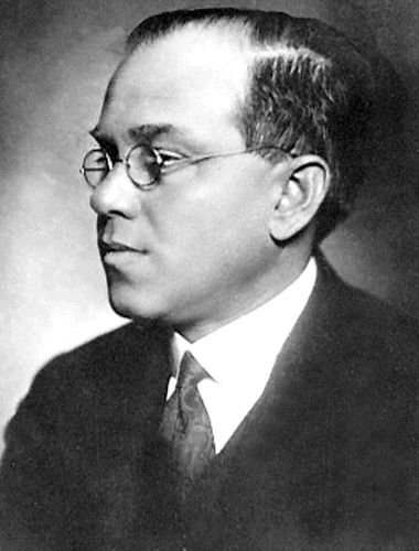
We are now primed to appreciate Fejér’s remarkable theorem that was proved in 1900 by a Hungarian mathematician Lipót Fejér (1880--1959). He was born into a Jewish family as Leopold Weiss. He spent 1899-1900 academic year at the University of Berlin, where Leopold attended courses by Georg Frobenius and Lazarus Fuchs, but it was his discussions with Hermann Schwarz that led him look at the convergence of Fourier series.

L. Fejér was the chair of mathematics at the University of Budapest since 1911 and led a highly successful Hungarian school of analysis. He was the thesis adviser of mathematicians such as John von Neumann, Paul Erdős, George Pólya, Marcel Riesz, Gábor Szegő, and Pál Turán.

Naturally, World War I had an impact on Lipót Fejér, to which a serious illness added in 1916. The effect of counterrevolutionary times was shown by a three-year gap in the list of his publication. However, as a Jew he suffered after the Nazis came to power. Fejér had a prostate operation in the early 1940s after which he did little research and, as a Jew, was forced to retire in 1944. On one December night 1944, the residents in his house on Tatra Street in Budapest were lined up before execution, but a brave officer saved their lives and dismissed the order. Although Fejér survived this horrific episode, his mental capacities rapidly deteriorated.

The following beautiful statement, proved by Fejér in 1900, asserts that the Fourier series is summable (C, 1) to the value of the function at each point of continuity.

Theorem (Lipót Fejér, 1900): Let \( f\,: \,[-\ell , \ell ]\, \mapsto \,\mathbb{R} \) be a continuous function with \( f(-\ell )= f(\ell ) . \) Then the Fourier series of f (C,1)-converges to f in \( C([-\ell , \ell ], \mathbb{R}) , \) where \( C([-\ell , \ell ], \mathbb{R}) \) is the metric space of continuous functions from \( [-\ell , \ell ] \) to the set of real numbers.

Lemma 1: The following trigonometric identity holds:
\[ \sin \frac{x}{2} + \sin \frac{3x}{2} + \cdots + \sin \left( n - \frac{1}{2} \right) x = \frac{\sin^2 \frac{nx}{2}}{\sin \frac{x}{2}} . \]
From identity \( \sin \left( k - \frac{1}{2} \right) x\,\sin\frac{x}{2} = \frac{1}{2} \left[ \cos (k-1) x - \cos kx \right] , \) it follows
\begin{align*} \sin\frac{x}{2}\,\sum_{k=1}^n \sin \left( k - \frac{1}{2} \right) x &= \frac{1}{2} \sum_{k=1}^n \left[ \cos (k-1)x - \cos kx \right] \\ &= \frac{1}{2} \left[ 1 - \cos nx \right] = \sin^2 \frac{nx}{2} . \end{align*}
Therefore,
\[ \sum_{k=1}^n \sin \left( k - \frac{1}{2} \right) x = \frac{\sin^2 \frac{nx}{2}}{\sin\frac{x}{2}} . \]
Lemma 2: Let \( S_n (x) = \frac{a_0}{2} + \sum_{k=1}^n a_k \cos kx + b_k \sin kx \) be the partial sum of the Fourier series of f(x). Let \( \sigma_n = \frac{1}{n} \left[ S_0 + S_1 (x) + \cdots + S_{n-1} (x) \right] \) be the partial Cesàro sum. Then
\[ \sigma_n (x) = \frac{1}{2\pi n} \int_0^{\pi} \left[ f(x+t) + f(x-t) \right] \left( \frac{\sin \frac{nt}{2}}{\sin\frac{t}{2}} \right)^2 {\text d}t . \]
Using identity for partial Fourier sums
\[ S_n (x) = \frac{1}{2\pi} \int_0^{\pi} \left[ f(x+t) + f(x-t) \right] \frac{\sin \left( n + \frac{1}{2} \right) t}{\sin\frac{t}{2}}\,{\text d}y , \]
Corollary: If f is integrable on some finite interval, then the Fourier series of f is Cesàro summable to f at every point of continuity of f. Moreover, if f is continuous on the interval, then the Fourier series of f is uniformly Cesàro summable to f.

Without imposing any additional conditions on f aside from being continuous and periodic, Fejér’s theorem shows that Fourier series can still achieve uniform convergence, granted that we instead of regular convergence consider the arithmetic means of partial Fourier sums.
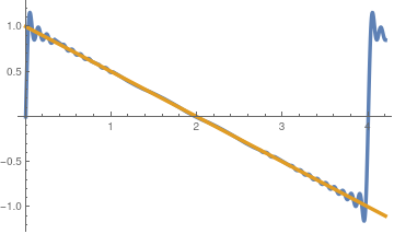
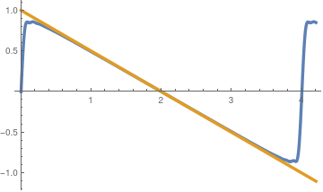
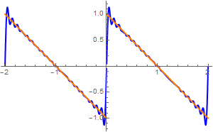
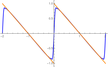
Example 3: Let us consider the function f(x) = sign(x) − x:

\[ f(x) = \frac{\ell -x}{2} = \frac{2}{\pi} \sum_{n\ge 1} \frac{1}{n}\,\sin \left( \frac{n \pi x}{\ell} \right) \qquad 0 < x < 2\ell . \]
Integrate[(1 - x/L)*Sin[n*Pi*x/L], {x, 0, L}]/L*2
(2 (n \[Pi] - Sin[n \[Pi]]))/(n^2 \[Pi]^2)
Its Cesàro partial sums are
\[ \sigma_N (x) = \sum_{n =1}^{N} \frac{1}{n}\left( 1 - \frac{n}{N} \right) \sin \left( \frac{n \pi x}{\ell} \right) = \sum_{n =1}^{N} \frac{1}{2n}\left( 1 - \frac{n}{N} \right) e^{{\bf j}n\pi x/\ell} - \sum_{n =1}^{N} \frac{1}{2n}\left( 1 - \frac{n}{N} \right) e^{-{\bf j}n\pi x/\ell} . \]
Its partial sums are expressed via special functions, so we prefer to make a numerical experiment.
            Using Mathematica, we plot Fourier partial sumes with 40 terms and then the corresponding Cesàro approximation.
C40[x_] = (2/Pi)*Sum[Sin[n*x*Pi/2]/n*(1 - n/40), {n, 1, 40}];
Plot[{S40[t], 1 - t/2}, {t, 0, 4.2}, PlotStyle -> Thickness[0.01]]
S40[x_] = (2/Pi)*Sum[Sin[n*x*Pi/2]/n, {n, 1, 40}];
Plot[{S40[t], 1 - t/2}, {t, 0, 4.2}, PlotStyle -> Thickness[0.01]]
       Fourier approximation with 40 terms.              Cesàro approximation with 40 terms.            Mathematica code

Upon plotting partial Fourier sum and Cesàro sum
\[ S_n (x) = \frac{2}{\pi} \, \sum_{k= 1}^n \frac{1}{k} \left( 1- \frac{k-1}{n} \right) \sin \left( k\pi x \right) , \]
with n = 20 terms, we don't observe Gibbs phenomenon in the latter one.
   

f[x_] := Sign[x] - x
bn=Integrate[f[x]*Sin[k*Pi*x], {x, -1, 1}]
sin[m_] = (2/Pi)*Sum[(1/k)*Sin[k*Pi*x], {k, 1, m}]
cesin[m_] = (2/Pi)*Sum[(1/k)*(1 - (k-1)/m)*Sin[k*Pi*x], {k, 1, m}]
Plot[{sin[20], f[x]}, {x, -2, 2}, PlotStyle -> {{Thick, Blue}, {Thick, Orange}}]
Plot[{cesin[20], f[x]}, {x, -2, 2}, PlotStyle -> {{Thick, Blue}, {Thick, Orange}}]
End of Example 3

A more general form of the theorem applies to functions which are not necessarily continuous. Suppose that f is absolutely integrable on the finite interval \( [-\ell , \ell ] . \) If the left and right limits \( f(x_0 \pm 0) \mbox{ of } f(x) \) exist at x0, or if both limits are infinite of the same sign, then

\[ \frac{1}{n}\,\sum_{k= 0}^{n-1} S_k = \sum_{k= 0}^{n-1} \left( 1- \frac{k}{n} \right) a_k \,\mapsto \, \frac{1}{2} \left[ f(x_0 +0) + f(x_0 -0) \right] \quad\mbox{as}\quad n \,\mapsto \infty . \]
Existence or divergence to infinity of the Cesàro mean is also implied. ■

Lemma: If f is integrable on the interval [-ℓ,ℓ], then Fourier series in Cesàro sense
\[ (C.1)\quad \sum_{k=-n}^n \alpha_k (f)\, e^{{\bf j}kx\pi /\ell} = \frac{1}{2\ell} \,\int_{-\ell}^{\ell} f(x-t)\, K_n (t)\,{\text d} t , \]
where
\[ K_n (t) = \frac{1}{n+1}\left( \csc \left( \frac{\pi t}{2\ell} \right) \sin \left( \frac{(n+1)\pi t}{2\ell} \right) \right)^2 = \sum_{k=-n}^n \left( 1 -\frac{|k|}{n+1} \right) e^{{\bf j}\pi kt /\ell}, \qquad t\ne 0, \]
is called the Fejér kernel. Also, Kn(0) = (n+1)-1.    ▣
Simplify[Assuming[x \[Element] Reals, Sum[(1 - Abs[k]/(1*n + 1))*Exp[I*x*Pi*k/L], {k, -n, n}]]]
(E^(-((I n \[Pi] x)/ L)) (-1 + E^((I (1 + n) \[Pi] x)/L))^2)/((-1 + E^((I \[Pi] x)/ L))^2 (1 + n))
Theorem 2: Let f ∈ 𝔏p(−ℓ, ℓ) be a periodic function with 1 ≤ p < ∞. Then Cesàro partial sums \( \sigma_n (f) = \sum_{k=-n}^n \left( 1 - \frac{|k|}{n+1} \right) \hat{f} (k)\, e^{{\bf j} k\pi x/\ell} \) converge to f(x) in 𝔏p sense:
\[ \lim_{n\to\infty} \left( \int_{-\ell}^{\ell} \left\vert \sigma_n (f) - f(x) \right\vert^p {\text d} x \right)^{1/p} = 0. \]
Indeed, we have
\[ \left( \int_{-\ell}^{\ell} \left\vert \sigma_n (f)(x) - f(x) \right\vert^p {\text d} x \right)^{1/p} = \left( \int_{-\ell}^{\ell} \left\vert \left( F_n \ast f \right) (x) - f(x) \right\vert^p {\text d} x \right)^{1/p} , \]
where
\[ F_n (x) = \frac{1}{n+1} \left( \frac{\sin \frac{\left( n+1 \right) \pi x}{2\ell}}{\sin \frac{\pi x}{2\ell}} \right)^2 \]
is the Fejér’s kernel and asterisk means convolution:
\[ \left( f \ast g \right) (x) = \int_{-\ell}^{\ell} f(t)\,g(x-t)\,{\text d}t = \int_{-\ell}^{\ell} f(x-t)\,g(t)\,{\text d}t . \]
Using the property
\[ \int_{-\ell}^{\ell} F_n (x)\,{\text d} x = 2\ell , \]
we rewrite the latter as
\begin{align*} \| F_n - f \|_p &= \left( \int_{-\ell}^{\ell} \left\vert \frac{1}{2\ell} \int_{-\ell}^{\ell} F_n (y) \left( f(x-y) - f(x) \right) {\text d}y \right\vert^p {\text d}x \right)^{1/p} \\ &\le \frac{1}{2\ell} \left( \int_{-\ell}^{\ell} \left\vert \int_{|y| < \delta} F_n (y) \left( f(x-y) - f(x) \right) {\text d}y \right\vert^p {\text d}x \right)^{1/p} + \frac{1}{2\ell} \left( \int_{-\ell}^{\ell} \left\vert \int_{|y| > \delta} F_n (y) \left( f(x-y) - f(x) \right) {\text d}y \right\vert^p {\text d}x \right)^{1/p} . \end{align*}
The first integral can be estimated as
\begin{align*} I_1 &= \frac{1}{2\ell} \left( \int_{-\ell}^{\ell} \left\vert \int_{|y| < \delta} F_n (y) \left( f(x-y) - f(x) \right) {\text d}y \right\vert^p {\text d}x \right)^{1/p} \\ & \le \frac{1}{2\ell} \int_{|y|< \delta} F_n (y) \left( \int_{-\ell}^{\ell} \left\vert f(x-y) - f(x) \right\vert^p {\text d}x \right)^{1/p} {\text d}y \\ & \le \sup_{|y| < \delta} \left( \int_{-\ell}^{\ell} \left\vert f(x-y) - f(x) \right\vert^p {\text d}x \right)^{1/p} \frac{1}{2\ell} \int_{|y| < \delta} F_n (y) \,{\text d}y \\ &= \sup_{|y| < \delta} \left( \int_{-\ell}^{\ell} \left\vert f(x-y) - f(x) \right\vert^p {\text d}x \right)^{1/p} \to 0 \qquad \delta \to 0. \end{align*}
The second integral can be estimated as well,
\begin{align*} I_2 &= \frac{1}{2\ell} \left( \int_{-\ell}^{\ell} \left\vert \int_{\delta < |y| < \ell} F_n (y) \left( f(x-y) - f(x) \right) {\text d}y \right\vert^p {\text d}x \right)^{1/p} {\text d} y \\ &\le \frac{1}{2\ell} \int_{\delta < |y| < \ell} F_n (y)\,{\text d} y \left( \int_{-\ell}^{\ell} \left\vert f(x-y) - f(x) \right\vert^p {\text d} x \right)^{1/p} \\ &\le 2 \left( \int_{-\ell}^{\ell} \left\vert f(x) \right\vert^p {\text d} x \right)^{1/p} \frac{1}{2\ell} \int_{\delta < |y| < \ell} F_n (y) {\text d} y , \end{align*}
where f is assumed to be periodic. The next step is to note for ℓ = π that
\[ \sin^2 \frac{y}{2} \ge \left( \frac{2}{\pi}\,\frac{|y|}{2} \right)^2 \ge \left( \frac{\delta}{\pi} \right)^2 \]
for π ≥ |y| > δ. That is why we have
\[ F_n (y) \le \frac{1}{n+1} \cdot \frac{1}{\sin^2 \frac{y}{2}} \le \frac{1}{n+1} \cdot \frac{\pi^2}{\delta^2} . \]
Hence
\[ \frac{1}{2\ell} \int_{\delta < |y| < \ell} F_n (y)\,{\text d} y \le \frac{\pi^2}{2\pi \delta^2} \cdot \frac{2 \left( \pi - \delta \right)}{n+1} \lt; \frac{\pi^2}{\sqrt{n}} \to 0 \]
as n → ∞ if we choose \( \delta = n^{-1/4} . \)
Example 4: Let f be the periodic function defined on the interval [-1,1]:
\[ f(x) = \begin{cases} 0 , & \quad \mbox{if $x\in (-1, -1/2)$, } \\ 1 , & \quad \mbox{if $x\in (-1/2, 1/2)$, } \\ 0 , & \quad \mbox{if $x\in (1/2, 1)$. } \end{cases} \]
Expanding this even function into Fourier series, we get
\[ f(x) = \frac{1}{2} + \frac{2}{\pi} \, \sum_{k\ge 1} \frac{1}{k} \, \sin \left( \frac{k\pi}{2} \right) \cos \left( k\pi x \right) = \frac{1}{2} - \frac{2}{\pi} \, \sum_{k\ge 1} \frac{(-1)^k}{2k-1} \, \cos \left( (2k-1)\pi x \right) ; \]
because
\[ \sin \left( \frac{k\pi}{2} \right) = \begin{cases} 0 , & \ \mbox{ if $k$ is even}, \\ (-1)^{k-1} , & \ \mbox{ if $k$ is odd}. \end{cases} \]
We can also expand the given function into complex Fourier series
\[ f(x) = \lim_{N\,\to \,\infty}\sum_{k=-N}^N \alpha_k \,e^{k{\bf j}\pi x} , \qquad \alpha_k = \frac{1}{2} \,\int_{-1}^1 f(x) \, e^{-k{\bf j}\pi x} \,{\text d}x = \frac{1}{k\pi} \,\sin \frac{k\pi}{2} , \quad k=0,\pm 1, \pm 2, \ldots . \]
Since f(0) = 1, we have
\[ \sum_{k\ge 1} \frac{1}{k} \, \sin \left( \frac{k\pi}{2} \right) = \sum_{n\ge 1} \frac{1}{2n-1} \, \sin \left( n\pi - \frac{\pi}{2} \right) = - \sum_{n\ge 1} \frac{1}{2n-1} \, \cos \left( n\pi \right) = \sum_{n\ge 1} \frac{(-1)^{n+1}}{2n-1} = \frac{\pi}{4} . \]
For each above Fourier series, we form the corresponding Cesàro partial sums
\begin{align*} C_m &= \frac{1}{2} + \frac{2}{\pi} \, \sum_{k= 1}^m \frac{1}{k} \left( 1- \frac{k}{m+1} \right) \sin \left( \frac{k\pi}{2} \right) \cos \left( k\pi x \right) , \quad m=1,2,\ldots ; \\ C_m &= \frac{1}{2} - \frac{2}{\pi} \, \sum_{k\ge 1} \frac{(-1)^k}{2k-1} \left( 1 - \frac{k}{m+1} \right) \cos \left( (2k-1)\pi x \right) , \quad m=1,2,\ldots ; \\ C_m &= \frac{1}{2} + \sum_{k=1}^m \left( 1 - \frac{k}{m+1} \right) \frac{1}{k\pi} \,\sin \left( \frac{k\pi}{2} \right) e^{{\bf j} k\pi x} + \frac{1}{k\pi} \left( 1 - \frac{k}{m+1} \right) \sin \left( \frac{k\pi}{2} \right) e^{-{\bf j} k\pi x} . \end{align*}
Plotting partial sums with n = 20 terms for Fourier series and Cesàro one, we don't see Gibbs phenomenon in Cesàro partial sums:
   

f[x_] := Piecewise[{{0, -1 < x < -1/2}, {1, -1/2 < x < 1/2}, {0, 1/2 < x < 1}}]
alphak = (1/2)*Integrate[Exp[I*k*Pi*x], {x, -1/2, 1/2}]]
an = Integrate[Cos[k*Pi*x], {x, -1/2, 1/2}]
cos[m_] = 1/2 + (2/Pi)* Sum[(1/k)*Sin[k*Pi/2]*Cos[k*Pi*x], {k, 1, m}]
cecos[m_] = 1/2 + (2/Pi)* Sum[(1/k)*(1 - k/(m + 1))*Sin[k*Pi/2]*Cos[k*Pi*x], {k, 1, m}]
Plot[{cecos[20], f[x]}, {x, -2, 2}, PlotStyle -> {{Thick, Blue}, {Thick, Orange}}]
When we plot these partial sums, we get exactly the same graphs:
alphak = Assuming[x \[Element] Reals, Integrate[f[x]*Exp[-k*Pi*I*x], {x, -1, 1}]/2 ]
complex[m_] = Sum[alphak*Exp[k*Pi*I*x], {k, -m, m}]
cesaro[m_] = 1/2 + Sum[alphak*Exp[k*Pi*I*x]*(1 - Abs[k]/(m + 1)), {k, 1, m}] + Sum[alphak*Exp[k*Pi*I*x]*(1 - Abs[k]/(m + 1)), {k, -m, -1}]
Plot[{cesaro[10]}, {x, -3, 3}, PlotStyle -> {Thick, Red}]
Example 5: Let (x) be the following piecewise continuous function on interval(−2, 2):
\[ f(x) = \begin{cases} x-\tfrac{1}{2} , & \ \mbox{ for} \quad 0 < x < 2, \\ a , & \ \mbox{ for} \quad -2 < x < 0 , \end{cases} \tag{5.1} \]
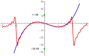
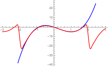
where 𝑎 is a real number that will be used to demonstrate the values of undershoots and overshoots of the corresponding Fourier series. It is convenient to represent the given function as the sum of two functions
\[ f(x) = f_{-} (x) + f_{+} (x) , \]
where
\[ f_{-}(x) = \begin{cases} 0, & \ \mbox{ for} \quad 0 < x < 2, \\ a , & \ \mbox{ for} \quad -2 < x < 0 , \end{cases} \qquad\mbox{and} \qquad f_{+}(x) = \begin{cases} x-\tfrac{1}{2} , & \ \mbox{ for} \quad 0 < x < 2, \\ 0, & \ \mbox{ for} \quad -2 < x < 0 , \end{cases} \tag{5.2} \]
Expanding these two auxiliary functions into sine-Fourier series, we get
f[x_] = Piecewise[{{a, -2 < x < 0}, {x - 1/2, 0 < x < 2}}]; a[n_] = 1/2*Integrate[f[x]*Cos[n*Pi*x/2], {x, -2, 2}]
(-4 + 4 Cos[n \[Pi]] + 3 n \[Pi] Sin[n \[Pi]] + 2 a n \[Pi] Sin[n \[Pi]])/(2 n^2 \[Pi]^2)
b[n_] = 1/2*Integrate[f[x]*Sin[n*Pi*x/2], {x, -2, 2}]
(-n \[Pi] - 2 a n \[Pi] - 3 n \[Pi] Cos[n \[Pi]] + 2 a n \[Pi] Cos[n \[Pi]] + 4 Sin[n \[Pi]])/(2 n^2 \[Pi]^2)
\[ f_{-}(x) = \frac{a}{2} + a \sum_{n\ge 1} \frac{(-1)^n -1}{n\pi}\,\sin \left( \frac{n\pi x}{2} \right) = \frac{a}{2} - \frac{2a}{\pi} \sum_{k\ge 1} \frac{1}{2k-1} \sin \left( \frac{(2k-1)\pi x}{2} \right) \tag{5.3} \]
and
\begin{align*} f_{+}(x) &= \frac{1}{4} + 2 \sum_{n\ge 1} \frac{(-1)^n -1}{n^2 \pi^2} \,\cos \left( \frac{n\pi x}{2} \right) - \frac{1}{2} \,\sum_{n\ge 1} \frac{3(-1)^n + 1}{n\pi}\,\sin \left( \frac{n\pi x}{2} \right) \\ &= \frac{1}{4} - \frac{4}{\pi^2} \sum_{k\ge 1} \frac{1}{(2k-1)^2}\,\cos \left( \frac{(2k-1)\pi x}{2} \right) - \frac{1}{\pi} \sum_{k\ge 1} \frac{1}{2k-1}\,\sin \left( \frac{(2k-1)\pi x}{2} \right) - \frac{1}{\pi} \sum_{k\ge 1} \frac{1}{k}\,\sin \left( k\pi x \right) . \tag{5.4} \end{align*}
We first check our answers with Parsevals' identity. For function f-(x), we have
\[ \frac{1}{2} + \frac{4}{\pi^2}\,\sum_{k\ge 1} \frac{1}{(2k-1)^2} = \frac{1}{2}\,\| f_{-} \|_2^2 = 1. \]
It is well-known that \( \sum_{k\ge 1} \frac{1}{(2k-1)^2} = \frac{\pi^2}{8} . \)
Sum[1/(2*k - 1)^2 , {k, 1, 100}]*8/Pi^2;
N[%]
0.997974
For function f+(x), we have
\[ \frac{1}{8} + \frac{16}{\pi^4} \sum_{k\ge 1} \frac{1}{(2k-1)^4} + \frac{1}{\pi^2} \,\sum_{k\ge 1} \frac{1}{(2k-1)^2} + \frac{1}{\pi^2} \sum_{k\ge 1} \frac{1}{k^2} = \frac{1}{2}\,\| f_{+} \|_2^2 = \frac{7}{12} \tag{5.5} \]
Using well-known identities
\[ \sum_{k\ge 1} \frac{1}{(2k-1)^2} = \frac{\pi^2}{8}, \qquad \sum_{k\ge 1} \frac{1}{k^2} = \frac{\pi^2}{6}, \qquad \sum_{k\ge 1} \frac{1}{(2k-1)^4} = \frac{\pi^4}{96} , \tag{5.6} \]
N[Sum[1/k^2, {k, 1, 100}]*6/Pi^2]
0.993951
Sum[1/(2*k - 1)^4 , {k, 1, 50}]*96/Pi^4;
N[%]
1.0
the equation (5.5) becomes
\[ \frac{16}{96} + \frac{1}{8} + \frac{1}{6} = \frac{7}{12} - \frac{1}{8} = \frac{11}{24} , \]
which is true.

Now we plot corresponding Fourier approximations that obtained by truncating the infinite series.

s30p[x_] = 1/4 - 4/Pi^2 *Sum[Cos[(2*k - 1)*Pi*x/2]/(2*k - 1)^2, {k, 1, 30}] - 1/Pi *Sum[Sin[(2*k - 1)*Pi*x/2]/(2*k - 1), {k, 1, 30} ] - 1/Pi*Sum[Sin[k*Pi*x]/k, {k, 1, 30}];
s30m[x_] = 1/2 - 2/Pi *Sum[Sin[(2*k - 1)*Pi*x/2]/(2*k - 1), {k, 1, 30}];
Plot[s30p[x] + s30m[x], {x, -3, 3}, PlotStyle -> Thick]
WE repeat calculations using
c30p[x_] = 1/4 - 4/Pi^2 * Sum[(1 - k/31)*Cos[(2*k - 1)*Pi*x/2]/(2*k - 1)^2, {k, 1, 30}] - 1/Pi *Sum[(1 - (k - 1)/30)*Sin[(2*k - 1)*Pi*x/2]/(2*k - 1), {k, 1, 30} ] - 1/Pi*Sum[(1 - (k - 1)/30)*Sin[k*Pi*x]/k, {k, 1, 30}];
c30m[x_] = 1/2 - 2/Pi * Sum[(1 - (k - 1)/30)*Sin[(2*k - 1)*Pi*x/2]/(2*k - 1), {k, 1, 30}];
Plot[c30p[x] + c30m[x], {x, -3, 3}, PlotStyle -> Thick]


Fourier approximation with 30 terms.


Cesàro approximation with 30 terms.
Example 6: Let \( f(x) = 4x^3 -3x^2 -6x \) on the interval [-2,2]. Expanding this function into Fourier series, we get
\[ f(x) = -4 - \frac{8}{\pi^3} \, \sum_{k\ge 1} \left[ 6\pi k \,\cos \frac{k\pi x}{2} + \left( 5 k^2 \pi^2 -48 \right) \sin \frac{k\pi x}{2} \right] \frac{(-1)^k}{k^3} \]
because
f[x_] = 4*x^3 - 3*x^2 - 6*x
a0=Integrate[f[x], {x, -2, 2}]/2
ak=Integrate[f[x]*Cos[k*Pi*x/2]/2, {x, -2, 2}]
bk=Integrate[f[x]*Sin[k*Pi*x/2]/2, {x, -2, 2}]
fourier[m_]:=-4+Sum[ak*Cos[k*Pi*x/2] + bk*Sin[k*Pi*x/2], {k,1,m}]
We build Fourier and Cesàro approximations and then plot partial sums with n = 20 terms:
   

cesaro[m_] := -4 + Sum[(ak*Cos[k*Pi*x/2] + bk*Sin[k*Pi*x/2])*(1 - k/(m + 1)), {k, 1, m}]
pp = Plot[{f[x], fourier[20]}, {x, -3, 3}, PlotStyle -> {{Thick, Blue}, {Thick, Red}}, Epilog -> {Text[11.58, {-.66, 11.579}], Text[-35.58, {-.66, -35.58}]}]
p = Graphics[{Green, PointSize[Large], {Point[{0, 11.57959}], Point[{0, -35.58}]}}]
Show[pp, p]
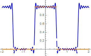
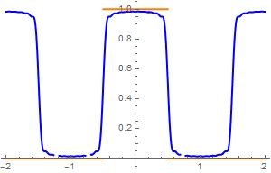
The Fourier graph clearly displays the Gibbs phenomenon at points of discontinuity x = 2 and x = -2. Since \( f(2+0) = -32 \quad\mbox{and}\quad f(2-0) =8 , \) the given function has finite jump of 40 at both points of discontinuity. Therefore, we expect overshoot/undershoot by the value \( (1.1789797444721675*40 - 40)/2 \approx 3.579594889 . \) As a result, we expect overshoot at points of discontinuity to be about 11.57959 and undershoot to be around -35.5796. Notably, we do not observe the Gibbs phenomenon in the Cesaro approximation.
  1. Fejér, L., Sur les fonctions intégrables et bornées, Comptes Rendus de l'Académie des Sciences, 1900, Vol. 131, 10 décembre 1900, pp. 984--987.
  2. Fejér, L., Untersuchungen über Fouriersche Reihen, Mathematische Annalen, 1904, vol. 58, pp. 51--69.


Return to Mathematica page
Return to the main page (APMA0340)
Return to the Part 1 Matrix Algebra
Return to the Part 2 Linear Systems of Ordinary Differential Equations
Return to the Part 3 Non-linear Systems of Ordinary Differential Equations
Return to the Part 4 Numerical Methods
Return to the Part 5 Fourier Series
Return to the Part 6 Partial Differential Equations
Return to the Part 7 Special Functions