Return to computing page for the first course APMA0330
Return to computing page for the second course APMA0340
Return to Mathematica tutorial for the first course APMA0330
Return to Mathematica tutorial for the second course APMA0340
Return to the main page for the first course APMA0330
Return to the main page for the second course APMA0340
Return to Part II of the course APMA0340
Introduction to Linear Algebra with Mathematica
Glossary
Planar Phase Portrait
Consider a systems of linear differential equations with constant coefficients
Since we know the structure of solutions to Eq.\eqref{EqPhase.1} from its fundamental matrix \( e^{{\bf A}\,t} , \) it is expected that the analysis of solutions near the origin is the most fruitful. It is not a surprise that this case requires a special attention.
Recall that a neighborhood of a point p is any set in ℝn that contains an open ball \( \| {\bf x} - {\bf p} \| = \sqrt{\left( x_1 - p_1 \right)^2 + \cdots +\left( x_n - p_n \right)^2 } < \varepsilon \) centered at p = [p1, …, pn]T. An equilibrium (also called stationary) solution of the autonomous system \eqref{EqPhase.2} is a point where the derivative of \( {\bf x}(t) \) is zero. An equilibrium solution is a constant solution of the system, and is usually called a critical point. For a linear system \( \dot{\bf x} = {\bf A}\,{\bf x}, \) an equilibrium solution occurs at each solution of the system (of homogeneous algebraic equations) \( {\bf A}\,{\bf x} = {\bf 0} . \) As we have seen, such a system has exactly one solution, located at the origin, if \( \det{\bf A} \ne 0 .\) If \( \det{\bf A} = 0 , \) then there are infinitely many solutions, and the critical point is not isolated.
Previously, we used a direction (or tangent) field to depict the behavior of solutions without actual solving the differential equation. Now we are going to enhance its features by adding arrows to accommodate time presence and plot some typical solutions. The accurate tracing of the parametric curves of the solutions is not an easy task without computers. However, we can obtain a very reasonable approximation of a trajectory by using the very same idea behind the slope field, namely the tangent line approximation.
We will classify the critical points of various systems of first order linear differential equations by their stability. Since the general treatment of stability and instability is given in Part III of this tutorial, it is reasonable to provide its descriptive definition.
In addition, due to the truly two-dimensional nature of the parametric curves, we will also classify the type of those critical points based on the behavior of solutions near equilibria (or, rather, by the shape formed by the trajectories about each critical point).
In our study of phase portraits and critical points, we will encounter four types of critical points: nodes, saddle point, spiral, and center. Note that this is typical only for two-dimensional problems. Additionally, these critical points are based on the eigenvalues and eigenvectors of the constant coefficient linear system of differential equations. The table below emphasizes the relationship between the stability and type of critical point based on the eigenvalues.
Singular Matrices
Example 1: Consider the 2×2 matrix
Eigenvalues[A]
|
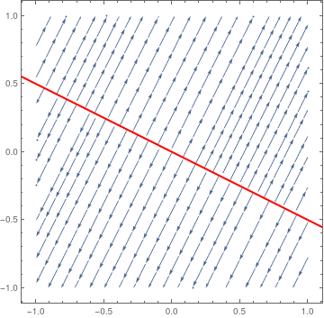
So we know that the eigenvalue λ = 0 has a corresponding eigenvector [−2, 1]. Then we plot the direction field along with the separatrix corresponding to the eigenspace of λ = 0.
sp = StreamPlot[{x + 2*y, 2*x + 4*y}, {x, -1, 1}, {y, -1, 1}];
line = Graphics[{Thick, Red, Line[{{-2, 1}, {2, -1}}]}]; Show[sp, line] |
|
| Separatrix is an example of non-isolated equilibria. | Mathematica code |
■
Isolated Equilibria
As a rule, we will only consider systems of linear differential equations whose coefficient matrix A has a nonzero determinant.
In two-dimensional space, it is possible to completely classify the critical points of various systems of first order linear differential equations by their stability. In addition, due to the truly two-dimensional nature of the parametric curves, we will also classify the type of those critical points by their shapes (or, rather, by the shape formed by the trajectories about each critical point). Their classification is based on eigenvalues of the coefficient matrix. Therefore, we consider different cases.
There are four types of critical points. To characterize them, it is convenient to use polar coordinates. Suppose that the solution curve of the autonomous planar differential equation dx/dt = f(x) can be written as x = x(t), y = y(t), where x = [x(t), y(t)]T is a two-dimensional column vector. Then in polar coordinates, their trajectory can be written as
Nodes
- proper node or star when every semi-line from the critical point is a tangent to some orbit;
- improper node when there are at most two directions along which trajectories approach the critical point;
- degenerate node when there is only one direction along which orbits approach the critical point.
For constant coefficient linear differential equations, classification of critical points can be performed based on eigenvalues of the corresponding constant matrix.
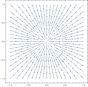
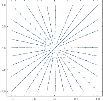
Case 1: Diagonal real-valued matrix with the same entries and of the same sign. A proper node can be observed only when the matrix of the system is a constant real multiple of the diagonal matrix:
Example 2: Consider the following 2×2 matrices
VectorPlot[{x, 2*y}, {x, -1, 1}, {y, -1, 1}, PlotTheme -> "Scientific"]
StreamPlot[{-x, -y}, {x, -1, 1}, {y, -1, 1}, StreamPoints -> 30]
VectorPlot[{-x, -2*y}, {x, -1, 1}, {y, -1, 1}, PlotTheme -> "Web"]
|
|
||
| Figure 2: Proper nodal source, matrix A1. | Figure 3: Proper nodal sink, matrix A2. |
Case 2: Distinct real eigenvalues of the same sign. Then the general solution of the linear system \( \dot{\bf x} = {\bf A}\,{\bf x}, \) is
where \( \lambda_1 \) and \( \lambda_2 \) are distinct real eigenvalues, \( {\bf \xi} \) and \( {\bf \eta} \) are corresponding eigenvectors, and \( c_1 , c_2 \) are arbitrary real constants.
When eigenvalues λ1 and λ2 are both positive, or are both negative, the phase portrait shows trajectories either moving away from the critical point toways infinity (for positive eigenvalues), or moving directly towards and converging to the critical point (for negative eigenvalues). The trajectories that are the eigenvectors move in straight lines. The rest of the trajectories move, initially when near the critical point, roughly in the same direction as the eigenvector of the eigenvalue with the smaller absolute value. Then, farther away, they would bend toward the direction of the eigenvector of the eigenvalue with the larger absolute value. This type of critical point is called a node. It is asymptotically stable if eigenvalues are both negative, unstable if eigenvalues are both positive.
Stability: It is unstable if both eigenvalues are positive; asymptotically stable if they are both negative.
Example 3: We start with the diagonal matrix and corresponding autonomous differential equation
|
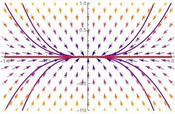
We plot the direction field along with some trajectories and separatrix
y = 0. Another eigenspace x = 0 (vertical line) is not actually a separatrix, and it is not shown.
vp = VectorPlot[{x, 2*y}, {x, -1, 1}, {y, -1, 1}, PlotTheme -> "Scientific"];
tb = Plot[Table[c*x^2, {c, -2, 2}], {x, -1, 1}, PlotStyle -> {Thick, Purple}, PlotRange -> {-1, 1}]; line = Graphics[{Red, Thickness[0.01], Line[{{-1, 0}, {1, 0}}]}]; Show[tb, vp, line] Mathematica code. |
|
| Separatrix y = 0 (in red) and phase portrait for matrix B. The origin is a nodal source---repeller. |
For another diagonal matrix
|
Upon separation of variables, we obtain its general solution
\[ \frac{{\text d}y}{{\text d}x} = \frac{\dot{y}}{\dot{x}} = \frac{-3y}{-x} \qquad \Longrightarrow \qquad y = x^3 . \]
We plot the direction field along with some trajectories and separatrix
y = 0
vp = VectorPlot[{-x, -3*y}, {x, -1, 1}, {y, -1, 1}, PlotTheme -> "Scientific"];
tb = Plot[Table[c*x^2, {c, -2, 2}], {x, -1, 1}, PlotStyle -> {Thick, Purple}, PlotRange -> {-1, 1}]; line = Graphics[{Red, Thickness[0.01], Line[{{-1, 0}, {1, 0}}]}]; Show[tb, vp, line] |
|
| Separatrix y = 0 (in red) and phase portrait for matrix B2. The origin is a nodal sink (attractor). | Mathematica code |
■
Example 4: Consider two matrices
Eigenvalues[A1]
arr1a = Graphics[{Red, Thick, Arrowheads[0.06], Arrow[{{1, 1}, {0.1, 0.1}}]}];
arr2 = Graphics[{Purple, Thick, Arrowheads[0.06], Arrow[0.5*{{1, 2}, {0.2, 0.4}}]}];
arr4 = Graphics[{Purple, Thick, Arrowheads[0.06], Arrow[0.5*{{-1, -2}, {-0.2, -0.4}}]}];
arr3 = Graphics[{Red, Thick, Arrowheads[0.06], Arrow[{{-1, -1}, {0, 0}}]}];
arr3a = Graphics[{Red, Thick, Arrowheads[0.06], Arrow[{{-1, -1}, {-0.1, -0.1}}]}];
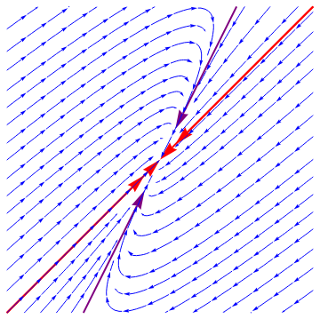
sp = StreamPlot[{-5*x + 2*y, -4*x + y}, {x, -1, 1}, {y, -1, 1}, PlotTheme -> "Scientific", StreamStyle -> Blue];
Show[arr1, arr1a, arr2, arr3, arr3a, arr4, sp]
Now we perform a similar job with another matrix A2.
Eigenvalues[A2]
arr1 = Graphics[{Red, Thick, Arrowheads[0.06], Arrow[{{0, 0}, {1, 1}}]}];
arr1a = Graphics[{Red, Thick, Arrowheads[0.06], Arrow[{{0, 0}, {0.9, 0.9}}]}];
arr2 = Graphics[{Orange, Thick, Arrowheads[0.06], Arrow[{{0, 0}, {-1, 1}}]}];
arr4 = Graphics[{Orange, Thick, Arrowheads[0.06], Arrow[{{0, 0}, {1, -1}}]}];
arr3 = Graphics[{Red, Thick, Arrowheads[0.06], Arrow[{{0, 0}, {-1, -1}}]}];
arr3a = Graphics[{Red, Thick, Arrowheads[0.06], Arrow[{{0, 0}, {-0.9, -0.9}}]}];
Show[arr1, arr1a, arr2, arr3, arr3a, arr4, vp]
|
|
|
| Figure 6: Improper nodal source with dominated separatrix labeled by double arrow. | Figure 7: Improper nodal sink. |
Case 3: Repeated real eigenvalue with one eigenvector. If a square 2×2 matrix is not diagonal and has a defective (repeated) eigenvalue, then the matrix has only one eigenvector. It is not diagonalizable and its general solution is of the form
Example 5: Consider two matrices
Eigenvalues[A3]
line = Graphics[{Red, Thick, Line[{{-1, -1}, {1, 1}}]}];
Show[line, vp]
Eigenvalues[A3]
line = Graphics[{Red, Thickness[0.01], Line[{{-1, 1}, {1, -1}}]}];
Show[line, sp]
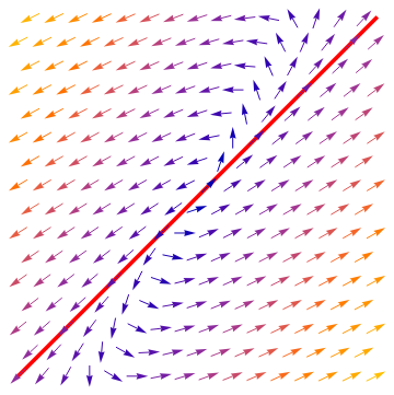
|
|
|
| Figure 8: Degenerate nodal source. | Figure 9: Degenerate nodal sink. |
Saddle points
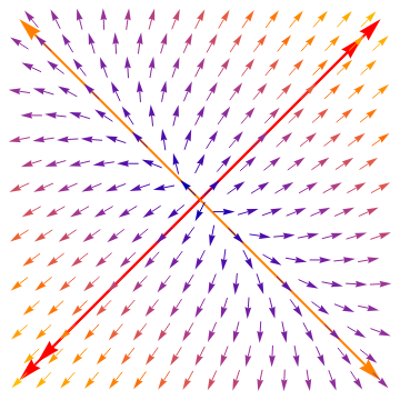
Case 4: Distinct real eigenvalues are of opposite signs. In this type of phase portrait, the trajectories given by the eigenvectors of the negative eigenvalue initially start at infinity before moving towards and eventually converging at the critical point. The trajectories that represent the eigenvectors of the positive eigenvalue move in exactly the opposite way: starting at the critical point before diverging to infinity. Every other trajectory starts at infinity, moves toward but never converges to the critical point, and then changes direction and moves back towards infinity. All the while it would roughly follow the 2 sets of eigenvectors. This type of critical point is called a saddle point. It is always unstable.
Stability: It is always unstable.
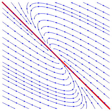
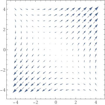
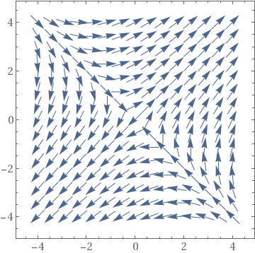
Example 6: Consider a system of ordinary differential equations
The coefficient matrix
\( {\bf A} = \begin{bmatrix} 1&2 \\ 2&1 \end{bmatrix} \)
has two distinct real eigenvalues
\( \lambda_1 =3 \) and
\( \lambda_2 =-1 . \) Therefore, the critical point, which is the origin, is a saddle point, unstable. We plot the corresponding phase portrait using the following codes.
Mathematica provides us at least two options: either
StreamPlot or VectorPlot (for the latter we give two versions without normalization and with it).
Manipulate[ Show[splot, ParametricPlot[ Evaluate[ First[{x[t], y[t]} /.
NDSolve[{x'[t] == x[t] + 2*y[t], y'[t] == 2*x[t] + y[t], Thread[{x[0], y[0]} == point]}, {x, y}, {t, 0, T}]]], {t, 0, T}, PlotStyle -> Red]], {{T, 20}, 1, 100}, {{point, {3, 0}}, Locator}, SaveDefinitions -> True]
VectorPlot
| StreamPlot | VectorPlot | VectorPlot with normalization |
|---|---|---|
|
|
|
Spiral points
- all trajectories are defined on t0 < t < ∞ or −∞ < t < t0 for some t0;
- \( \lim_{t\to +\infty} r (t) = 0 \) or \( \lim_{t\to -\infty} r (t) = 0 . \)
- \( \lim_{t\to +\infty} \left\vert \omega (t) \right\vert = \infty \) or \( \lim_{t\to -\infty} \left\vert \omega (t) \right\vert = \infty . \)
Case 5: Complex conjugate eigenvalues. When the real part of eigenvalues is nonzero, the trajectories still retain the elliptical traces. However, with each revolution, their distances from the critical point grow/decay exponentially according to the term \( e^{\Re\lambda\,t} , \) where \( \Re\lambda \) is the real part of the complex λ, the eigenvalue. Therefore, the phase portrait shows trajectories that spiral away from the critical point toways infinity (when \( \Re\lambda > 0 \) ), or trajectories that spiral toward, and converge to the critical point (when \( \Re\lambda < 0 \) ). This type of critical point is called a spiral point. It is asymptotically stable if \( \Re\lambda < 0 ,\) it is unstable if \( \Re\lambda > 0 . \)
An example of a stable spiral is provided by the underdamped oscillator: \( \ddot{x} + \dot{x} + x = 0 . \)Example 7: Consider two matrices
|
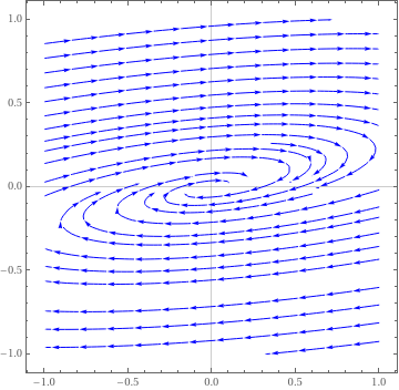
We plot the direction field in a neighborhood of the asymptotically stable stationary point. Note that trajectories approach the origin in clockwise direction.
StreamPlot[{-3*x + 13*y, -x + y}, {x, -1, 1}, {y, -1, 1}, PlotTheme -> "Scientific", StreamStyle -> Blue, PerformanceGoal -> "Quality", StreamPoints -> 25]
|
|
| Spiral critical point for matrix A6. | Mathematica code |
|
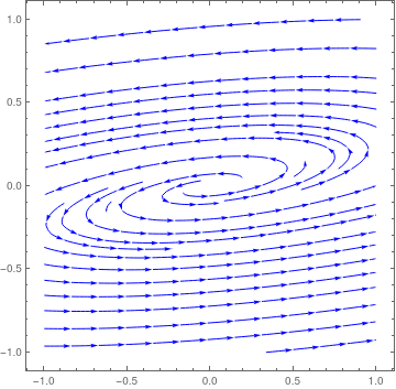
We plot the direction field in a neighborhood of the asymptotically stable stationary point for matrix −A6. Note that trajectories approach the origin in counterclockwise direction.
StreamPlot[{3*x - 13*y, x - y}, {x, -1, 1}, {y, -1, 1}, PlotTheme -> "Detailed", StreamStyle -> Blue, PerformanceGoal -> "Quality", StreamPoints -> 25]
|
|
| Spiral asymptotically stable critical point for matrix −A6. | Mathematica code |
Now we do a similar job for matrix A5 that has unstable critical point at the origin.
|
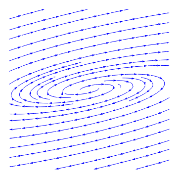
We plot the direction field in a neighborhood of the ustable stationary point. Note that trajectories depart from the origin in clockwise direction.
StreamPlot[{-x + 13*y, -x + 3*y}, {x, -1, 1}, {y, -1, 1}, PlotTheme -> "Minimal", StreamStyle -> Blue, PerformanceGoal -> "Quality", StreamPoints -> 25]
|
|
| Spiral unstable critical point for matrix A5. | Mathematica code |
|
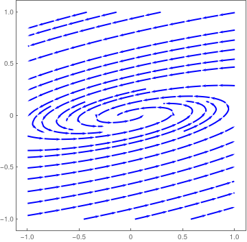
We plot the direction field in a neighborhood of the unstable stationary point for matrix −A5. Note that trajectories depart from the origin in counterclockwise direction.
StreamPlot[{x - 13*y, x - 3*y}, {x, -1, 1}, {y, -1, 1}, PlotTheme -> "Web", StreamStyle -> Blue, PerformanceGoal -> "Quality", StreamPoints -> 25]
|
|
| Spiral unstable critical point for matrix −A5. | Mathematica code |
■
Center
Case 6: Two pure complex conjugate eigenvalues. When the real part of the eigenvalues is zero, the trajectories neither converge to the critical point nor move toways infinitey. Rather, they stay in constant, elliptical (or, rarely, circular) orbits. This type of critical point is called a center. It has a unique stability classification shared by no other: stable (or neutrally stable).
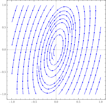
An example of a center is provided by the simple harmonic oscillator: \( \ddot{x} + x = 0 . \)Example 8: Consider the system of differential equations
|
We plot the direction field.
StreamPlot[{x -y, 5*x - y}, {x, -1, 1}, {y, -1, 1}, PlotTheme -> "Scientific", StreamStyle -> Blue, PerformanceGoal -> "Quality", StreamPoints -> 25]
|
|
| Center critical point. | Mathematica code |
■
| Eigenvalues | Condition | Type of Critical Point | Stability |
|---|---|---|---|
| λ1 > λ2 > 0 | tr(A) > 0 and tr²(A) > 4 det(A), det(A) > 0 | Nodal source (node) | Unstable |
| λ1 < λ2 < 0 | tr(A) < 0 and tr²(A) > 4 det(A), det(A) > 0 | Nodal sink (node) | Asymptotically stable |
| λ1 < 0 < λ2 | detA < 0 | Saddle point | Unstable |
| λ1 = λ2 > 0 diagonal matrix |
A = k I with k>0 | Proper node (star) | Unstable |
| λ1 = λ2 < 0 diagonal matrix |
A = k I with k<0 | Proper node (star) | Asymptotically stable |
| λ1 = λ2 > 0 missing eigenvector |
A = k1 I + k2 I with k>0 | Improper/degenerate node | Unstable |
| λ1 = λ2 < 0 missing eigenvalue |
A = k1 I + k2 I with k<0 | Improper/degenerate node | Asymptotically stable |
| λ = α ± jβ, α > 0 | tr(A) > 0 and tr²(A) < 4 det(A) | Spiral point | Unstable |
| λ = α ± jβ, α < 0 | tr(A) < 0 and tr²(A) < 4 det(A) | Spiral point | Asymptotically stable |
| λ = ± jβ | tr(A) = 0 and tr²(A) < 4 det(A) | Center | Stable |
Mathematica plots phase portraits
Mathematica gives several options to plot phase portraits for planar systems of differential equations. We show them by examples. Matrix
Eigenvalues[c]
|
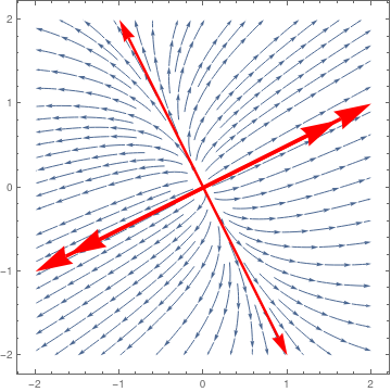
Then we plot direction field and two separatrices using StreamPlot
ar1 = Graphics[{Red, Thickness[0.01], Arrowheads[0.1], Arrow[{{0, 0}, {2, 1}}]}];
ar1a = Graphics[{Red, Thickness[0.01], Arrowheads[0.1], Arrow[{{0, 0}, {1, 0.5}*1.6}]}]; ar2 = Graphics[{Red, Thickness[0.01], Arrowheads[0.1], Arrow[{{0, 0}, {-2, -1}}]}]; ar2a = Graphics[{Red, Thickness[0.01], Arrowheads[0.1], Arrow[{{0, 0}, {-1, -0.5}*1.6}]}]; ar3 = Graphics[{Red, Thickness[0.007], Arrowheads[0.06], Arrow[{{0, 0}, {-1, 2}}]}]; ar3a = Graphics[{Red, Thickness[0.007], Arrowheads[0.06], Arrow[{{0, 0}, {1, -2}}]}]; sp = StreamPlot[{13 x + 4 y, 4 x + 7 y}, {x, -2, 2}, {y, -2, 2}]; Show[sp, ar1, ar1a, ar2, ar2a, ar3, ar3a] |
|
| Nodal repeller and two separatreces. | Mathematica code |
|
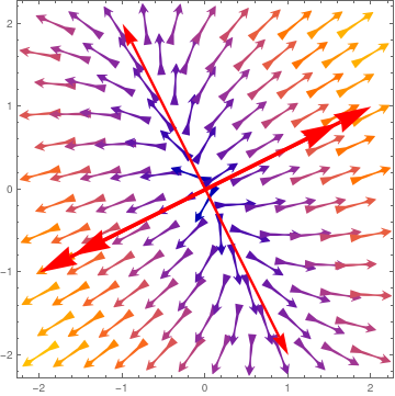
Then we plot the direction field with VectorPlot command. As usual, the dominated eigenspace is identified with double arrow.
ar1 = Graphics[{Red, Thickness[0.01], Arrowheads[0.1], Arrow[{{0, 0}, {2, 1}}]}];
ar1a = Graphics[{Red, Thickness[0.01], Arrowheads[0.1], Arrow[{{0, 0}, {1, 0.5}*1.6}]}]; ar2 = Graphics[{Red, Thickness[0.01], Arrowheads[0.1], Arrow[{{0, 0}, {-2, -1}}]}]; ar2a = Graphics[{Red, Thickness[0.01], Arrowheads[0.1], Arrow[{{0, 0}, {-1, -0.5}*1.6}]}]; ar3 = Graphics[{Red, Thickness[0.007], Arrowheads[0.06], Arrow[{{0, 0}, {-1, 2}}]}]; ar3a = Graphics[{Red, Thickness[0.007], Arrowheads[0.06], Arrow[{{0, 0}, {1, -2}}]}]; vp = VectorPlot[{13 x + 4 y, 4 x + 7 y}, {x, -2, 2}, {y, -2, 2}, VectorScale -> 0.1, VectorPoints -> 12, VectorStyle -> "Dart"]; Show[vp, ar1, ar1a, ar2, ar2a, ar3, ar3a] |
|
| Two Separatrices divide the phase plane into four parts. | Mathematica code |
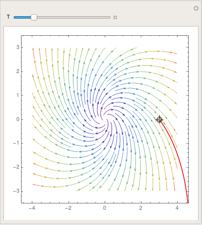
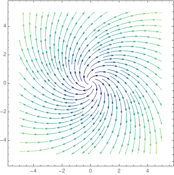
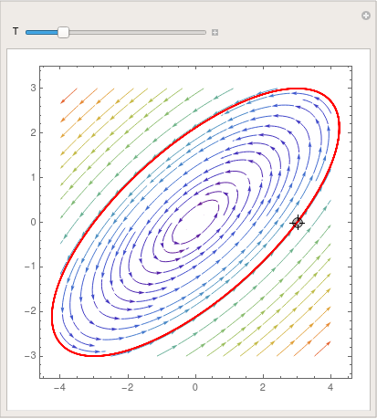
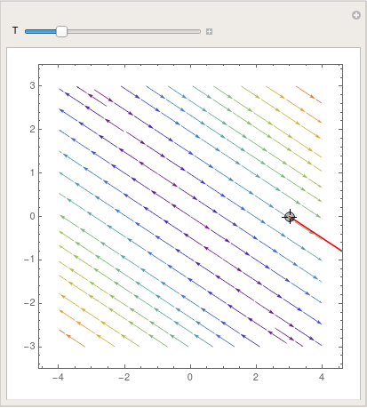
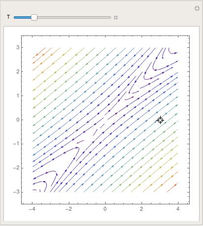
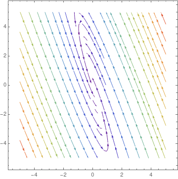
We can take advantage of the Manipulate command that allows one to change
(in our case) the initial point along with the direction field:
|
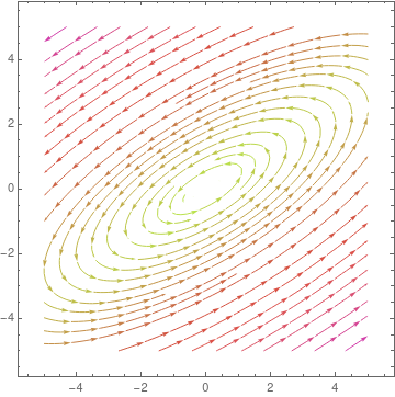
parta = StreamPlot[{x + y, y - x}, {x, -4, 4}, {y, -3, 3},
StreamColorFunction -> "Rainbow"]; Manipulate[ Show[parta, ParametricPlot[ Evaluate[ First[{x[t], y[t]} /. NDSolve[{x'[t] == x[t] + y[t], y'[t] == y[t] - x[t], Thread[{x[0], y[0]} == point]}, {x, y}, {t, 0, T}]]], {t, 0, T}, PlotStyle -> Red]], {{T, 20}, 1, 100}, {{point, {3, 0}}, Locator}, SaveDefinitions -> True] |
|
| Demonstration of Manipulate command. | Mathematica code |
To save the image, use Mathematica command Export:
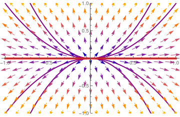
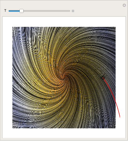
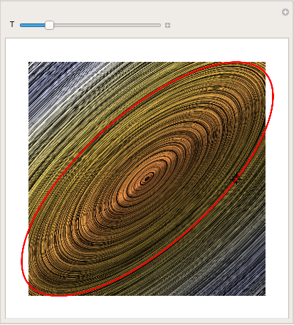
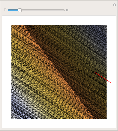
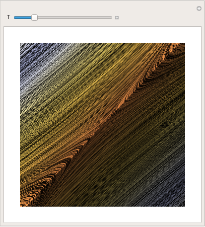
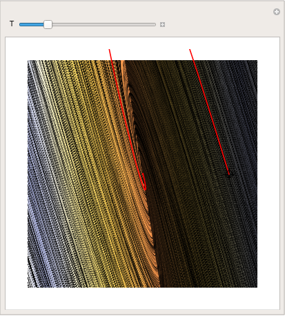
You can even make a cool picture by using LineIntegralConvolutionPlot:
|
parta = LineIntegralConvolutionPlot[{{x + y, y - x}, {"noise", 1000,
1000}}, {x, -4, 4}, {y, -3, 3}, ColorFunction -> "BeachColors", LightingAngle -> 0, LineIntegralConvolutionScale -> 3, Frame -> False]; Manipulate[ Show[parta, ParametricPlot[ Evaluate[ First[{x[t], y[t]} /. NDSolve[{x'[t] == x[t] + y[t], y'[t] == y[t] - x[t], Thread[{x[0], y[0]} == point]}, {x, y}, {t, 0, T}]]], {t, 0, T}, PlotStyle -> Red]], {{T, 20}, 1, 100}, {{point, {3, 0}}, Locator}, SaveDefinitions -> True] |
|
| Demonstration of LineIntegralConvolutionPlot command. | Mathematica code |
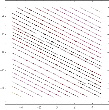
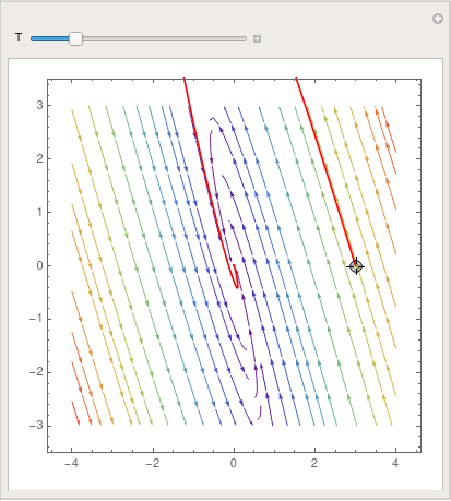
To put three colors into the plot, one may use
StreamColorFunction -> "Rainbow"];
Manipulate[
Show[partb,
ParametricPlot[
Evaluate[
First[{x[t], y[t]} /.
NDSolve[{x'[t] == x[t] - 2*y[t], y'[t] == -y[t] + x[t],
Thread[{x[0], y[0]} == point]}, {x, y}, {t, 0, T}]]], {t, 0,
T}, PlotStyle -> Red]], {{T, 20}, 1, 100}, {{point, {3, 0}},
Locator}, SaveDefinitions -> True]
To save the image as gif-file, type:
4}, {y, -3, 3}, ColorFunction -> "BeachColors",
LightingAngle -> 0, LineIntegralConvolutionScale -> 3,
Frame -> False];
Manipulate[
Show[partb,
ParametricPlot[
Evaluate[
First[{x[t], y[t]} /.
NDSolve[{x'[t] == x[t] - 2*y[t], y'[t] == -y[t] + x[t],
Thread[{x[0], y[0]} == point]}, {x, y}, {t, 0, T}]]], {t, 0,
T}, PlotStyle -> Red]], {{T, 20}, 1, 100}, {{point, {3, 0}},
Locator}, SaveDefinitions -> True]
StreamColorFunction -> "Rainbow"];
Manipulate[
Show[partc,
ParametricPlot[
Evaluate[
First[{x[t], y[t]} /.
NDSolve[{x'[t] == 2*x[t] + 2*y[t], y'[t] == -y[t] - x[t],
Thread[{x[0], y[0]} == point]}, {x, y}, {t, 0, T}]]], {t, 0,
T}, PlotStyle -> Red]], {{T, 20}, 1, 100}, {{point, {3, 0}},
Locator}, SaveDefinitions -> True]
1000}}, {x, -4, 4}, {y, -3, 3}, ColorFunction -> "BeachColors",
LightingAngle -> 0, LineIntegralConvolutionScale -> 3,
Frame -> False];
Manipulate[
Show[partc,
ParametricPlot[
Evaluate[
First[{x[t], y[t]} /.
NDSolve[{x'[t] == 2*x[t] + 2*y[t], y'[t] == -y[t] - x[t],
Thread[{x[0], y[0]} == point]}, {x, y}, {t, 0, T}]]], {t, 0,
T}, PlotStyle -> Red]], {{T, 20}, 1, 100}, {{point, {3, 0}},
Locator}, SaveDefinitions -> True]
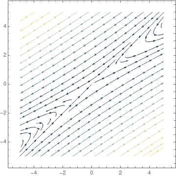
StreamPlot[{2*x + 2*y, -x - y}, {x, -5, 5}, {y, -5, 5},
StreamColorFunction -> "PlumColors"]
StreamColorFunction -> "Rainbow"];
Manipulate[
Show[partd,
ParametricPlot[
Evaluate[
First[{x[t], y[t]} /.
NDSolve[{x'[t] == 5*x[t] - 6*y[t], y'[t] == 3*x[t] - 4*y[t],
Thread[{x[0], y[0]} == point]}, {x, y}, {t, 0, T}]]], {t, 0,
T}, PlotStyle -> Red]], {{T, 20}, 1, 100}, {{point, {3, 0}},
Locator}, SaveDefinitions -> True]
1000}}, {x, -4, 4}, {y, -3, 3}, ColorFunction -> "BeachColors",
LightingAngle -> 0, LineIntegralConvolutionScale -> 3,
Frame -> False];
Manipulate[
Show[partd,
ParametricPlot[
Evaluate[
First[{x[t], y[t]} /.
NDSolve[{x'[t] == 5*x[t] - 6*y[t], y'[t] == 3*x[t] - 4*y[t],
Thread[{x[0], y[0]} == point]}, {x, y}, {t, 0, T}]]], {t, 0,
T}, PlotStyle -> Red]], {{T, 20}, 1, 100}, {{point, {3, 0}},
Locator}, SaveDefinitions -> True]
StreamPlot[{5*x - 6*y, 3*x - 4*y}, {x, -5, 5}, {y, -5, 5},
StreamColorFunction -> "StarryNightColors"]
StreamColorFunction -> "Rainbow"];
Manipulate[
Show[parte,
ParametricPlot[
Evaluate[
First[{x[t], y[t]} /.
NDSolve[{x'[t] == -4*x[t] - y[t], y'[t] == 2*y[t] + 10*x[t],
Thread[{x[0], y[0]} == point]}, {x, y}, {t, 0, T}]]], {t, 0,
T}, PlotStyle -> Red]], {{T, 20}, 1, 100}, {{point, {3, 0}},
Locator}, SaveDefinitions -> True]
1000}}, {x, -4, 4}, {y, -3, 3}, ColorFunction -> "BeachColors",
LightingAngle -> 0, LineIntegralConvolutionScale -> 3,
Frame -> False];
Manipulate[
Show[parte,
ParametricPlot[
Evaluate[
First[{x[t], y[t]} /.
NDSolve[{x'[t] == -4*x[t] - 1*y[t], y'[t] == 10*x[t] + 2*y[t],
Thread[{x[0], y[0]} == point]}, {x, y}, {t, 0, T}]]], {t, 0,
T}, PlotStyle -> Red]], {{T, 20}, 1, 100}, {{point, {3, 0}},
Locator}, SaveDefinitions -> True]
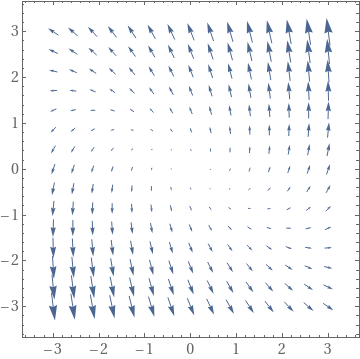
There is another way to visualize solutions to vector differential e quation---use VectorPlot :
Show[VectorPlot[A.{x, y}, {x, -3, 3}, {y, -3, 3}], Frame -> True,
BaseStyle -> {FontFamily -> "Times", FontSize -> 14}]
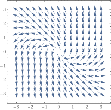
If one wants to see equal size arrows, type:
A.{x, y}/(10^-8 + Norm[A.{x, y}]), {x, -3, 3}, {y, -3, 3}],
Frame -> True, BaseStyle -> {FontFamily -> "Times", FontSize -> 14}]
A2 = {{-1, 2}, {-5, 5}};
A3 = {{1, -6}, {6, 1}};
A4 = {{-1, -2}, {1, 1}};
A5 = {{-1, -4}, {2, -5}};
A6 = {{1, -4}, {1, 5}};
A7 = {{2, -4}, {3, -5}};
Alist = {A1, A2, A3, A4, A5, A6, A7}; (*List of the different matrices*)
(*The below loop evaluates the relative signs of the eigenvalues, and \ then determines what type of critical points and stability it has. *)
Do[Print[ i, " " ];
If[(Eigenvalues[Alist[[i]]][[1]] > 0 && Eigenvalues[Alist[[i]]][[2]] > 0) && (Eigenvalues[Alist[[i]]][[ 2]] != Eigenvalues[Alist[[i]]][[1]]), Print["a) Nodal Source"]; Print["b) Unstable"]];
If[(Eigenvalues[Alist[[i]]][[1]] < 0 && Eigenvalues[Alist[[i]]][[2]] < 0) && (Eigenvalues[Alist[[i]]][[ 2]] !=E igenvalues[Alist[[i]]][[1]]), Print[ "a) Nodal Sink"]; Print[ "b) Asymptotically stable"]];
If[(Eigenvalues[Alist[[i]]][[1]] > 0 && Eigenvalues[Alist[[i]]][[2]] < 0) || (Eigenvalues[Alist[[i]]][[1]] < 0 && Eigenvalues[Alist[[i]]][[2]]> 0), Print["a) Saddle Point"]; Print["b) Unstable"]];
If[(Eigenvalues[Alist[[i]]][[1]] > 0 && Eigenvalues[Alist[[i]]][[2]] == Eigenvalues[Alist[[i]]][[1]]) && (Eigenvectors[Alist[[i]]][[ 1]] == Eigenvectors[Alist[[i]]][[2]]), Print["a) Proper Node/Star Point"]; Print["b) Unstable"]];
If[(Eigenvalues[Alist[[i]]][[1]] < 0 && Eigenvalues[Alist[[i]]][[2]]==E igenvalues[Alist[[i]]][[1]]) && (Eigenvectors[Alist[[i]]][[ 1]]==E igenvectors[Alist[[i]]][[2]]), Print[ "a) Proper Node/Star Point"]; Print[ "b) Asymptotically Stable"]];
If[(Eigenvalues[Alist[[i]]][[1]] > 0 && Eigenvalues[Alist[[i]]][[2]] == Eigenvalues[Alist[[i]]][[1]]) && (Eigenvectors[Alist[[i]]][[ 1]] != Eigenvectors[Alist[[i]]][[2]]), Print["a) Improper/Degenerate Node"]; Print["b) Unstable"]];
If[(Eigenvalues[Alist[[i]]][[1]] < 0 && Eigenvalues[Alist[[i]]][[2]]==E igenvalues[Alist[[i]]][[1]]) && (Eigenvectors[Alist[[i]]][[ 1]] !=E igenvectors[Alist[[i]]][[2]]), Print[ "a) Improper/Degenerate Node"]; Print[ "b) Asymptotically Stable"]];
If[Re[Eigenvalues[Alist[[i]]][[1]]] > 0 && Im[Eigenvalues[Alist[[i]]][[1]]] != 0, Print["a) Spiral Point"]; Print["b) Unstable"]];
If[Re[Eigenvalues[Alist[[i]]][[1]]] < 0 && Im[Eigenvalues[Alist[[i]]][[1]]] !=0 , Print[ "a) Spiral Point"]; Print[ "b) Asymptotically Zero"]];
If[Re[Eigenvalues[Alist[[i]]][[1]]] == 0 && Im[Eigenvalues[Alist[[i]]][[1]]] != 0, Print["a) Center"]; Print["b) Stable"]];
Print["c)"]; StreamPlot[{Alist[[i]][[1, 1]]*x + Alist[[i]][[1, 2]]*y, Alist[[i]][[2, 1]]*x + Alist[[i]][[2, 2]]*y}, {x, -3, 3}, {y, -3, 3}, StreamSyle->Fine] // Print, {i, 1, Legnth[Alist]}];
Return to Mathematica page
Return to the main page (APMA0340)
Return to the Part 1 Matrix Algebra
Return
to the
Part 2 Linear Systems of Ordinary Differential Equations
Return to the Part 3 Non-linear Systems of Ordinary Differential Equations
Return
to the
Part 4 Numerical Methods
Return to the Part 5 Fourier Series
Return to the Part 6 Partial Differential
Equations
Return to the Part 7 Special Functions