Preface
This tutorial was made solely for the purpose of education and it was designed for students taking Applied Math 0340. It is primarily for students who have some experience using Mathematica. If you have never used Mathematica before and would like to learn more of the basics for this computer algebra system, it is strongly recommended looking at the APMA 0330 tutorial. As a friendly reminder, don't forget to clear variables in use and/or the kernel. The Mathematica commands in this tutorial are all written in bold black font, while Mathematica output is in regular fonts.
Finally, you can copy and paste all commands into your Mathematica notebook, change the parameters, and run them because the tutorial is under the terms of the GNU General Public License (GPL). You, as the user, are free to use the scripts for your needs to learn the Mathematica program, and have the right to distribute this tutorial and refer to this tutorial as long as this tutorial is accredited appropriately. The tutorial accompanies the textbook Applied Differential Equations. The Primary Course by Vladimir Dobrushkin, CRC Press, 2015; http://www.crcpress.com/product/isbn/9781439851043
Return to computing page for the second course APMA0340
Return to Mathematica tutorial for the first course APMA0330
Return to Mathematica tutorial for the second course APMA0340
Return to the main page for the first course APMA0330
Return to the main page for the second course APMA0340
Return to Part III of the course APMA0340
Introduction to Linear Algebra
Glossary
Numerical Solutions
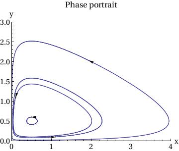
ParametricPlot[
Table[{x[t], y[t]} /. sol[[j]], {j, Length[ic]}], {t, 0, T},
PlotRange -> {{0, 4}, {0, 3}}],
Table[Graphics[{Arrowheads[.03],
Arrow[{ic[[j]], ic[[j]] + .01 f[ic[[j, 1]], ic[[j, 2]] ] }]}],
{j, Length[ic]}],
AxesLabel -> {"x", "y"},
BaseStyle -> {FontFamily -> "Times", FontSize -> 14},
PlotLabel -> "Phase portrait"
]
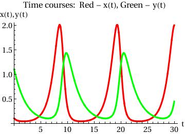
PlotStyle -> {{Thickness[0.01], RGBColor[1, 0, 0]}, {Thickness[0.01],
RGBColor[0, 1, 0]}}, AxesOrigin -> {0, 0},
AxesLabel -> {"t", "x(t),y(t)"},
BaseStyle -> {FontFamily -> "Times", FontSize -> 14},
PlotLabel -> "Time courses: Red - x(t), Green - y(t)"]
Example. Consider the system of autonomous equations
deq2 = y'[t] == 2*x[t]*y[t] - y[t]^2;
soln = NDSolve[{deq1, deq2, x[0] == 1, y[0] == 1}, {x[t], y[t]}, {t, -10, 10}];
Do[Clear[x, y];
soln = NDSolve[{deq1, deq2, x[0] == n/10, y[0] == n/10}, {x[t], y[t]}, {t, -10, 10}];
x = soln[[1, 1, 2]];
y = soln[[1, 2, 2]];
curve[[n]] = ParametricPlot[{x, y}, {t, -10, 10}, PlotStyle -> Thick], {n, -4, 4}];
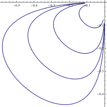
Show[curve[[-4]], curve[[-3]], curve[[-2]], curve[[-1]], curve[[1]], curve[[2]], curve[[3]], curve[[4]], AspectRatio -> 1]
soln = NDSolve[{deq1, deq2, x[0] == n/10, y[0] == n/10}, {x[t], y[t]}, {t, -10, 10}];
x = soln[[1, 1, 2]];
y = soln[[1, 2, 2]];
curvep[[n]] = ParametricPlot[{x, y}, {t, -10, 10}, PlotStyle -> Thick], {n, 0, 4}];
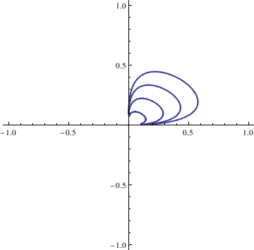
Show[curvep[[0]], curvep[[1]], curvep[[2]], curvep[[3]], curvep[[4]], AspectRatio -> 1]
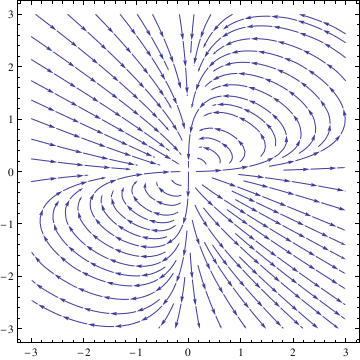
G[x_, y_] := x^3;
sol = NDSolve[{x'[t] == F[x[t], y[t]], y'[t] == G[x[t], y[t]],
x[0] == 1, y[0] == 0}, {x, y}, {t, 0, 3*Pi},
WorkingPrecision -> 20]
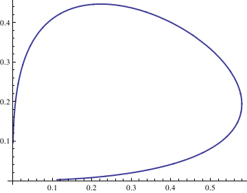
ParametricPlot[Evaluate[{x[t], y[t]}] /. sol, {t, 0, 3*Pi}]
Y[t_] := Evaluate[y[t] /. sol]
fns[t_] := {X[t], Y[t]};
len := Length[fns[t]];
Plot[Evaluate[fns[t]], {t, 0, 3*Pi}]
Return to Mathematica page
Return to the main page (APMA0340)
Return to the Part 1 Matrix Algebra
Return to the Part 2 Linear Systems of Ordinary Differential Equations
Return to the Part 3 Non-linear Systems of Ordinary Differential Equations
Return to the Part 4 Numerical Methods
Return to the Part 5 Fourier Series
Return to the Part 6 Partial Differential Equations
Return to the Part 7 Special Functions