Return to computing page for the second course APMA0340
Return to Mathematica tutorial for the first course APMA0330
Return to Mathematica tutorial for the second course APMA0340
Return to the main page for the first course APMA0330
Return to the main page for the second course APMA0340
Return to Part I of the course APMA0340
Introduction to Linear Algebra with Mathematica
Glossary
Mechanical Problems
Example 1: The following example is inspired by a phenomenon presented in Sutton's classical book (Demonstration Experiments in Physics, McGraw-Hill, New York, 1938) for demonstration that different points at a rigid rod pivoted at one end have distinct falling accelerations that can exceed the corresponding acceleration of the center of mass. Its analysis leads to determination of the center of percussion or center of oscillation of a rigid rod/stick (with respect to a particular axis of rotation)
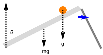
If we neglect friction, all freely falling point objects will fall at the acceleration of gravity, commonly called g. A ball is placed on one end of a uniform rod/stick , which is pivoted at the other end and makes initially an angle of about π/6 radians with the horizontal surface. The support of the elevated end of the stick is suddenly dropped, together with the ball. The falling end of the stick accelerates at a greater rate than the free-falling ball, proving that its acceleration is greater than g, the acceleration of gravity.
|
We plot the falling stick with a ball:
rod = Graphics[{LightGray,
Polygon[{{0, 0}, {-0.1, 0.1}, {1.9, 1.1}, {2.0, 1.0}}]}];
support = Graphics[{Gray, Thickness[0.02], Line[{{2.5, 0}, {2.0, 1.0}}]}]; ball = Graphics[{Orange, Disk[{1.5, 0.99}, 0.1]}]; ar = Graphics[{Blue, Thickness[0.02], Arrowheads[0.08], Arrow[{{1.9, 0.8}, {2.2, 0.8}}]}]; ar1 = Graphics[{Black, Dashed, Thickness[0.01], Arrowheads[0.08], Arrow[{{1, 0.5}, {1, 0}}]}]; ar2 = Graphics[{Black, Dashed, Thickness[0.01], Arrowheads[0.08], Arrow[{{0, 0}, {0, 1.2}}]}]; ar3 = Graphics[{Black, Dashed, Thickness[0.01], Arrowheads[0.08], Arrow[{{1.5, 0.99}, {1.5, 0.2}}]}]; t1 = Graphics[{Black, Text[Style["g", 18], {1.5, 0.1}]}]; t2 = Graphics[{Black, Text[Style["\[Theta]", 18], {0.15, 0.4}]}]; t3 = Graphics[{Black, Text[Style["mg", 18], {1.05, -0.1}]}]; Show[rod, support, ball, ar, ar1, ar2, ar3, t1, t2, t3] |
|
| Falling stick with a ball. | Mathematica code |
Let θ = θ(t) be the angular displacement of the rod from the vertical axis at time t, with θ0 = θ(0) defining the initial elevation of stick end. Suppose that the rod has length ℓ and mass m, with center of gravity at a distance of λℓ, from the hinge. The uniform rod has the moment of inertia around the axis at the hinge to be I0 = βmℓ². For the case of a thin uniform rod, λ = ½ and β = ⅓. Since any point object falls with a constant acceleration g ≈ 9.81, we can assume that the ball is of unit mass.
The equation for the rod along (without the ball) can be obtained by using Newton's second law for rotation around a fixed hinged point (which can be chosen as the origin) to give
The critical position of the ball is determined by α = α* when the acceleration of the point of its contact is equal to g. Since the acceleration of any point located at αℓ position is
However, the value (3.6) does not guarantee that the rod reaches the ground before the ball does. To calculate T from Eq.(1.4), we transfer the integral by substitution
- Adams, J.L., Acceleration greater than "g", The Physics Teacher, 1982, Issue 2, pp. 100--101; https://doi.org/10.1119/1.2340956
- Bacon, M.E., Harpst, M.R., and Nakazawa, R., Falling sticks and falling balls, The Physics Teacher, 2002, 40, 333–335 (Sept. 2002)
- Haber-Schaim, U., On qualitative problems, The Physics Teacher, 1992, 30, Issue 5, p. 260; https://doi.org/10.1119/1.2343533
- Härtel, H., The falling stick with 𝑎 > g, The Physics Teacher, 2000, 38, January, pp. 54--55. https://doi.org/10.1119/1.880430
- Hilton, W.A., Free fall paradox, The Physics Teacher, 1965, 3, Issue 7, pp. 323--324, https://doi.org/10.1119/1.2349174
- Shash, S., Shore, J.A., and Spekkens, K., The falling rod race, The Physics Teacher, 2020, 58, November, pp. 596--598; https://doi.org/10.1119/10.0002387
- Theron, W., The "faster than gravity" demonstration revisited, American Journal of Physics, 1988, 56, Issue 8, pp. 736--739. https://doi.org/10.1119/1.15513
- Varieschi, G, and Kamiya, K., Toy models for the falling chimney, American Journal of Physics, 2003, 71, No, 9, pp. 1025--1031. https://doi.org/10.1119/1.1576403
- Young, W.M., Faster than gravity!, American Journal of Physics, 1984, 52, No. 12, pp. 1142--1143. https://doi.org/10.1119/1.13745
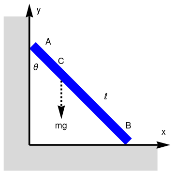
The sliding ladder paradox
We sketch the learning ladder with Mathematica:
ladder = Graphics[{Blue, Polygon[{{0, 1.5}, {0.1, 1.6}, {1.6, 0.1}, {1.5, 0}}]}];
ar1 = Graphics[{Black, Thickness[0.01], Arrowheads[0.08], Arrow[{{0, 0}, {2.2, 0}}]}];
ar2 = Graphics[{Black, Thickness[0.01], Arrowheads[0.08], Arrow[{{0, 0}, {0, 2.2}}]}];
ar3 = Graphics[{Black, Dashed, Thickness[0.01], Arrowheads[0.08], Arrow[{{0.5, 1}, {0.5, 0.4}}]}];
tl = Graphics[{Black, Text[Style["\[ScriptL]", 18, FontFamily -> "Mathematica1"], {1.2, 0.75}]}];
tx = Graphics[{Black, Text[Style["x", 18], {2.1, 0.2}]}];
ty = Graphics[{Black, Text[Style["y", 18], {0.15, 2.1}]}];
tA = Graphics[{Black, Text[Style["A", 18], {0.3, 1.6}]}];
tB = Graphics[{Black, Text[Style["B", 18], {1.55, 0.3}]}];
tC = Graphics[{Black, Text[Style["C", 18], {0.5, 1.3}]}];
t3 = Graphics[{Black, Text[Style["mg", 18], {0.5, 0.3}]}];
t4 = Graphics[{Black, Text[Style["\[Theta]", 18], {0.1, 1.2}]}];
Show[pol, ladder, ar1, ar2, ar3, t3, t4, tx, ty, tl, tA, tB, tC]
In 1744, L.Euler introduced the angular momentum (moment of momentum) A of a system of particles with respect to the fixed origin of an inertial frame
The system of particles is now assumed to be isolated. This implies that Fα is the resultant only of the forces that all the other particles exert on the αth particles. Hence,
Hoverver, the angular momentum can be understood in different way by taking the reference point at P instead of the origin:
If on other hand the angular momentum is understood as
- point P is the center of mass of the system;
- point P is unaccelerated (relative to an internal frame);
- the acceleration of point P is directed toward or away from the center of mass.
Hu has pointed out in 2011 that the equation of motion of a rolling body can also be derived without needing to know the forces acting at a point P being attached to the ground:
- Crawford, F.S., Moments to remember, American Journal of Physics, 1989, 57, Issue 2, pp. 177--
- Faucher, G., Fixed points in torque--angular momentum relations, American Journal of Physics, 1983, 51, Issue 8, pp. 758--759.
- Hu, B.Y-K., Rolling asymmetric discs on an inclined plane, European Journal of Physics, 2011, 32, pp. L51--L54. doi: 0.1088/0143-0807/32/6/L05
- Illarramendi, M.A. and del Rio Gaztelurrutia, T., Moments to be cautious of---relative versus absolute angular momentum, European Journal of Physics, 1995, 16, pp. 249
- Jensen, J.H., Rules for rolling as a rotation about the instanteneous pointof contact, European Journal of Physics, 2011, 32, Issue pp. 389--397.
- Jensen, J.H., Five ways of deriving the equation of motion rolling bodies, American Journal of Physics, 2012, 80, Issue , pp.
- McDonald, K.T., Comments on torque analysis, Joseph Henry Laboratories, Princeton University, Princeton, NJ 08544, 2019.
- Podolsky, B., Conservation of angular momentum, American Journal of Physics, 1966, 42, Issue 1, pp. 42--45.
- Rodriguez, L., Torque and the rate of change of angular momentum at an arbitrary point, American Journal of Physics, 2003, 71, Issue 11, pp. 1201--1203.
- Theron, W.F.D., On using moments around the instantaneous center of rotation,American Journal of Physics, 2009, 77, Issue 10, pp. 918
- Tiersten, M.S., Moments not to forget---The conditions for equating torque and rate of angular momentum around the instantaneous center, American Journal of Physics, 1991, 59, Issue 8, pp. 733--738.
- Tiersten, M.S., Erratum: Moments not to forget---The conditions for equating torque and rate of angular momentum around the instantaneous center, American Journal of Physics, 1992, 60, Issue , p. 187.
- Turner, L. and Turner, A.M., Asymmetric rolling bodies and the phantom torque, American Journal of Physics, 2010, 78, Issue 9, pp. 905--908. https://doi.org/10.1119/1.3456118
- Zypman, F.R., Moments to remember---The condition for equating torque and rate of change of angular momentum, American Journal of Physics, 1990, 58, Issue 1, pp. 41--43. https://doi.org/10.1119/1.16316
Example 2: Let a uniform rod ("ladder") of mass m and length 2ℓ is leaning against a wall at some angle. Suppose that it is released from the rest and slides in the xy-plane along a smooth wall and smooth floor.
In 1744, L.Euler introduced the angular momentum (moment of momentum) L with respect to the fixed origin of an inertial frame
Example 3: ■
- Freeman, M., Palffy-Muhoray, P., On mathematical and physical ladders, American Journal of Physics, 1985, 53, pp. 276--277.
- Kapranidis,S., Koo, R., Variations of the sliding ladder problem, The College Mathematics Journal, 2008, 39, No. 3, pp. 374--379.
- Majumdar, P.,Roy, M., Friction controlled three stage ladder sliding motion in an non-conservative system: From pre-detachment to post-detachment, The African Review of Physics, 2012,
- McDonald, K.T., Comments on torque analysis, 2019, Princeton University.
- McDonald, K.T., Torque analysis of a sliding ladder, 2019, Princeton University.
- Scholten, P., Simoson, A., The falling ladder paradox, The College Mathematics Journal, 1996, 27, pp. 49--54.
Rolling sphere
- Hu, Ben Yu-Kuang, Rolling asymmetric discs on an inclined plane, European Journal of Physics, 2011, 32, pp. L51--L54.
- McDonald, K.T., Cylinder rolling on another rolling cylinder, Joseph Henry Laboratories, Princeton University, Princeton, NJ 08544, 2018.
- McDonald, K.T., Cylinder rolling inside another rolling cylinder, Joseph Henry Laboratories, Princeton University, Princeton, NJ 08544, 2016.
- McDonald, K.T., Slab rolling on a rolling cylinder, Joseph Henry Laboratories, Princeton University, Princeton, NJ 08544, 2016.
- Romer, R.H., Motion of a sphere on a tolted turntable, American Journal of Physics, 1981, 49, Issue 10, pp. 985--986.
- Welner, K., Stable circular orbits of greelymoving balls on rotating discs, American Journal of Physics, 1979, 47, Issue 11, pp. 984--986.
Return to Mathematica page
Return to the main page (APMA0340)
Return to the Part 1 Matrix Algebra
Return to the Part 2 Linear Systems of Ordinary Differential Equations
Return to the Part 3 Non-linear Systems of Ordinary Differential Equations
Return to the Part 4 Numerical Methods
Return to the Part 5 Fourier Series
Return to the Part 6 Partial Differential Equations
Return to the Part 7 Special Functions