Preface


This sections presents examples of solving the Laplace and Helmholtz equations subject to the Dirichlet boundary conditions in rectangular coordinates. The Dirichlet problem goes back to George Green who studied the problem on general domains with general boundary conditions in his «An Essay on the Application of Mathematical Analysis to the Theories of Electricity and Magnetism», published in 1828.

Return to computing page for the first course APMA0330
Return to computing page for the second course APMA0340
Return to Mathematica tutorial for the first course APMA0330
Return to Mathematica tutorial for the second course APMA0340
Return to the main page for the first course APMA0330
Return to the main page for the second course APMA0340
Return to Part VI of the course APMA0340
Introduction to Linear Algebra with Mathematica


Let Ω be a subset of n-dimensional Euclidean spacen with a smooth boundary ∂Ω; let also \( L\left[ \texttt{D} \right] \) be a elliptic partial differential operator of the second order. There are known two Dirichlet problems: either interior or inner Dirichlet problem or exterior or outer Dirichlet problem. The inner problem asks to find a solution of elliptic equation \( L\left[ \texttt{D}\right] u = 0 \) inside the domain Ω given values on the boundary ∂Ω of Ω. The exterior Dirichlet problem asks for a solution outside the domain Ω subject the boundary conditions on ∂Ω. These two Dirichlet problems are also called first boundary value problem.
A typical example of an elliptic partial differential equation is Laplace's equation ∇²u = 0, and its solutions deserve a special name.
Solutions of Laplace's equation ∇²u = 0 are called potential functions or harmonic functions. The operator Δ = ∇·∇ = ∇² is called the Laplace operator or Laplacian. In the Cartesian coordinates, the Laplacian is written as \( \Delta = \frac{\partial^2}{\partial x_1^2} + \frac{\partial^2}{\partial x_2^2} + \cdots + \frac{\partial^2}{\partial x_n^2} . \)


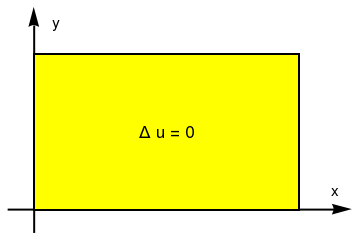
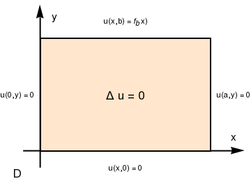
Consider the general planar Dirichlet problem for Laplace's equation

\begin{equation} \label{EqDirichlet.1} u_{xx} + u_{yy} =0 , \qquad 0 < x < a, \quad 0< y <b , \end{equation}
in the rectangle \( [0,a] \times [0,b] , \) and also satisfying the boundary conditions
\begin{equation} \label{EqDirichlet.2} u(x,0) = f_0 (x) , \qquad u(x,b) = f_b (x) , \qquad 0 < x < a, \end{equation}
and
\begin{equation} \label{EqDirichlet.3} u(0, x) = g_0 (y) , \qquad u(a,x) = g_a (y) , \qquad 0 < y < b, \end{equation}
where f0, fb, g0, and ga are given functions that are usually assumed to be square integrable (so belong to the space 𝔏²).
rectangle = Graphics[{EdgeForm[Thick], Yellow, Rectangle[{0, 0}, {3, 2}]}]
ax = {Arrowheads[Large], Arrow[{{-0.3, 0}, {3.6, 0}}]}
ax1 = Graphics[{Thick, Black, ax}]
ay = {Arrowheads[Large], Arrow[{{0, -0.3}, {0, 2.6}}]}
ay1 = Graphics[{Thick, Black, ay}]
txt1 = Graphics[Text[Style["x", FontSize -> 14], {3.4, 0.25}]]
txt2 = Graphics[Text[Style["y", FontSize -> 14], {0.25, 2.4}]]
right = Graphics[ Text[Style["u(x,b) = \!\(\*SubscriptBox[\(f\), \(b\)]\)[x]", Large], {4.3, 1}]]
delta = Graphics[ Text[Style["\[CapitalDelta] u = 0", FontSize -> 16], {1.5, 1.0}]]
Show[ax1, ay1, rectangle, txt1, txt2, delta, AspectRatio -> 2/3]
Domain for Dirichlet's problem.

Since the boundary of the rectangle has four corner points, we need to impose the requirement on the behavior of the solution in neighborhoods of each corner point to guarantee the uniqueness of the formulated boundary value problem. This topic is beyond the scope of the tutorial, so there are some references.

Also, in applications, it is required that boundary functions satisfy the regularity conditions:

\begin{equation} \label{EqDirichlet.4} g_0 (0) = f_0 (0) , \qquad g_a (0) = f_0 (a), \qquad g_a (b) = f_b (a) , \qquad g_0 (b) = f_b (0) . \end{equation}
These regularity conditions guarantee that the Dirichlet boundary value problem for the Laplace equation is well-posed. 
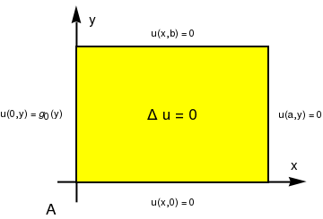
The first observation of the Dirichlet problem for Laplace's equation is that the partial differential equation is both linear and homogeneous, while the boundary conditions are only linear, but not homogeneous. Therefore, we cannot directly apply the separation of variable method because its application requires homogenization in one of the boundary value variables. Since we don't know any other solving method yet, we break the given problem into sum of four auxiliary problems that have homogeneous boundary conditions on each side of the rectangle except one. So we are going to solve four Dirichlet problems for Laplace's equation:
\[ u(x,y) = u_A (x,y) + u_B (x,y) + u_C (x,y) + u_D (x,y) . \]
Note that such decomposition into four Dirichlet problems may violate the regularity conditions; however, we ignore this issue for time being. The four problems are probably best shown with a quick sketch. Actually, the separation of variables requires representation of the solution as the sum of two functions
\[ u(x,y) = u_{AB} (x,y) + u_{CD} (x,y) , \qquad \mbox{where} \quad u_{AB} (x,y) = u_A (x,y) + u_B (x,y), \quad u_{CD} (x,y) = u_C (x,y) + u_D (x,y) . \]
Hence, the function uAB is the solution of the interior Dirichlet BVP:
\[ \Delta u = 0 \quad\mbox{insider the rectangle } (0,a)\times (0,b) \qquad\mbox{subject to} \quad u(0,y) = g_0 (x), \quad u(a,y) = g_a (y), \quad u(x,0) = u(x,b) = 0; \]
while function uCD is the solution of the interior Dirichlet BVP:
\[ \Delta u = 0 \quad\mbox{insider the rectangle } (0,a)\times (0,b) \qquad\mbox{subject to} \quad u(0,y) = u(a,y) = 0, \quad u(x,0) = f_0 (x), \quad u(x,b) = f_b (x) . \]
However, all calculations and formulas become simpler with separation of the given problem into four Dirichlet problems.

Completely similar decomposition of the given boundary value problem is valid for the exterior Dirichlet problem.

rectangle = Graphics[{EdgeForm[Thick], Yellow, Rectangle[{0, 0}, {3, 2}]}]
left = Graphics[ Text[Style["u(0,y) = \!\(\*SubscriptBox[\(g\), \(0\)]\)(y)"], {-0.7, 1}]]
aA = Graphics[Text[Style["A", FontSize -> 16], {-0.4, -0.4}]]
a0 = Graphics[Text[Style["u(x,0) = 0"], {1.5, -0.2}]]
a1 = Graphics[Text[Style["u(a,y) = 0"], {3.5, 1.0}]]
a2 = Graphics[Text[Style["u(x,b) = 0"], {1.5, 2.2}]]
Show[ax1, ay1, rectangle, txt1, txt2, delta, left, a0, a1, a2, aA, AspectRatio -> 3/4]
rectangleB = Graphics[{EdgeForm[Thick], Pink, Rectangle[{0, 0}, {3, 2}]}]
right = Graphics[ Text[Style["u(a,y) = \!\(\*SubscriptBox[\(g\), \(a\)]\)(y)"], {3.6, 1}]]
b1 = Graphics[Text[Style["u(0,y) = 0"], {-0.4, 1.0}]]
aB = Graphics[Text[Style["B", FontSize -> 16], {-0.4, -0.4}]]
Show[ax1, ay1, rectangleB, txt1, txt2, delta, right, a0, b1, a2, aB, AspectRatio -> 3/4]
rectangleC = Graphics[{EdgeForm[Thick], LightCyan, Rectangle[{0, 0}, {3, 2}]}]
down = Graphics[ Text[Style[ "u(x,0) = \!\(\*SubscriptBox[\(f\), \(0\)]\)(x)"], {1.5, -0.3}]]
c0 = Graphics[Text[Style["u(a,y) = 0"], {3.4, 1.0}]]
aC = Graphics[Text[Style["C", FontSize -> 16], {-0.4, -0.4}]]
Show[ax1, ay1, rectangleC, txt1, txt2, delta, down, c0, b1, a2, aC, AspectRatio -> 3/4]
rectangleD = Graphics[{EdgeForm[Thick], LightOrange, Rectangle[{0, 0}, {3, 2}]}]
top = Graphics[ Text[Style["u(a,y) = \!\(\*SubscriptBox[\(g\), \(a\)]\)(y)", Large], {0.5, 2.4}]]
aD = Graphics[Text[Style["D", FontSize -> 16], {-0.4, -0.4}]]
d2 = Graphics[Text[Style["u(a,y) = 0"], {3.4, 1.0}]]
Show[ax1, ay1, rectangleD, txt1, txt2, delta, top, a0, b1, d2, aD, AspectRatio -> 3/4]
                                                                 

Problem 1A: has homogeneous boundary conditions in variable y:

\[ u(0,y) = g_0 (y) , \quad u(a,y) =0, \quad u(x,0) =0, \quad u(x,b) =0. \]
We seek partial nontrivial solutions of the Laplace equation representing by the product of two functions \( u(x,y) = X(x)\,Y(y) \) and satisfying the homogeneous boundary conditions in y. Substituting u = X Y in the Laplace equation and separating variables, we obtain
\[ \frac{X'' (x)}{X(x)} = -\frac{Y'' (y)}{Y(y)} = \lambda , \]
where λ is the separation constant. Thus, we get the two ordinary differential equations
\[ \begin{split} X'' (x) + \lambda\,X(x) &= 0, \\ Y'' (y) + \lambda\, Y(y) &= 0 . \end{split} \]
From the homogeneous boundary conditions in y, it follows that
\[ Y(0) =0, \qquad Y(b) =0 . \]
So we get the Sturm--Liouville problem for variable Y(y): \( Y'' (y) + \lambda\, Y(y) = 0 , \quad Y(0) =0, \ Y(b) =0 . \) This problem is essentially identical to one encountered previously, and we conclude that the Sturm--Liouville problem has discrete number of eigenvalues
\[ \lambda_n = \left( \frac{n\pi}{b} \right)^2 , \qquad n=1,2,\ldots , \]
to which correspond eigenfunctions
\[ Y_n (y) = \sin \frac{n\pi y}{b} , \qquad n=1,2,\ldots . \]
Next, we substitute the eigenvalues into the differential equation for X(x), obtaining
\[ X'' (x) - \left( \frac{n\pi}{b} \right)^2 X(x) =0 , \qquad n=1,2,\ldots . \]
It is convenient to express its general solution in terms of hyperbolic functions instead of exponential functions:
\[ X(x) = c_1 \cosh \frac{n\pi x}{b} + c_2 \sinh \frac{n\pi x}{b} , \]
for some constant c1 and c2. Since the solution X(x) depends on n, we use the notation Xn(x) instead of X(x). The boundary condition X(𝑎) = 0 dictates
\[ X(a) = c_1 \cosh \frac{n\pi a}{b} + c_2 \sinh \frac{n\pi a}{b} =0 \qquad \Longrightarrow \qquad c_2 = - c_1 \,\mbox{coth} \frac{n\pi a}{b} . \]
Then the general solution for X(x)n(x) contains the only one arbitrary constant:
\[ X_n (x) = c_1 \cosh \frac{n\pi x}{b} - c_1 \,\mbox{coth} \frac{n\pi a}{b} \sinh \frac{n\pi x}{b} = c_1 \frac{1}{\sinh \frac{n\pi a}{b}} \left[ \sinh \frac{n\pi a}{b}\,\cosh \frac{n\pi x}{b} - \cosh \frac{n\pi a}{b}\,\sinh \frac{n\pi x}{b} \right] \]
Since \( \sinh (x-y) = \sinh x\,\cosh y - \cosh x \,\sinh y , \) , we simplify the expression for X:
\[ X_n (x) = \frac{c_1}{\sinh \frac{n\pi a}{b}} \, \sinh \left( \frac{n\pi}{b}(a-x) \right) . \]
Thus, we obtain partial nontrivial solutions (upon dropping an arbitrary constant multiplier)
\[ u_n (x,y) = \frac{1}{\sinh \frac{n\pi a}{b}} \, \sinh \left( \frac{n\pi}{b}(a-x) \right) \sin \frac{n\pi y}{b} , \qquad n=1,2,\ldots . \]
These functions satisfy the Laplace equation and two homogeneous boundary conditions in variable y for each value of n.

To satisfy the remaining nonhomogeneous boundary condition at x=0, we assume, as usual, that we can represent the solution as the sum of all partial nontrivial solutions:

\[ u(x,y) = \sum_{n\ge 1} c_n u_n (x,y) = \sum_{n\ge 1} \frac{c_n}{\sinh \frac{n\pi a}{b}} \, \sinh \left( \frac{n\pi}{b}(a-x) \right) \sin \frac{n\pi y}{b} . \]
The coefficients cn are determined by the boundary condition
\[ u(0,y) = \sum_{n\ge 1} c_n \, \frac{ \sinh \frac{n\pi a}{b}}{\sinh \frac{n\pi a}{b}} \, \sin \frac{n\pi y}{b} = \sum_{n\ge 1} c_n \, \sin \frac{n\pi y}{b} = g_0 (y) . \]
The quantities cn must be coefficients in the Fourier sine series of period 2b for g0:
\[ c_n = \frac{2}{b} \int_0^b g_0 (y) \,\sin \frac{n\pi y}{b} \,{\text d}y , \qquad n=1,2,\ldots . \]

To illustrate these formulae, let b=3a/4, and
\[ g_0 (y) = \begin{cases} y, & \ 0\le y \le 1, \\ \frac{a-y}{a-1} , & \ 1\le y \le b=\frac{3}{4}\,a . \end{cases} \]
Upon evaluating cn, we find that
\[ c_n = \frac{8}{3a} \int_0^{3a/4} g_0 (y) \,\sin \frac{4n\pi y}{3a} \,{\text d}y = \frac{9a^2 (a-2)}{16n\pi}\,\cos \frac{4n\pi}{3a} + \frac{27a^3}{32n^2 \pi^2}\,\sin \frac{4n\pi}{3a} - \frac{9a^3}{64n\pi}\,(-1)^n , \qquad n=1,2,\ldots . \]
c[n_,a_] := 3*a/4*Integrate[y*Sin[4*n*Pi*y/3/a], {y, 0, 1}, Assumptions -> Element[n, Integers]] ]
+ 3*a/4*Integrate[(a - y)*Sin[4*n*Pi*y/3/a], {y, 1, 3*a/4}, Assumptions -> Element[n, Integers]]
Keeping 10 terms in the series, we can plot u versus x and y, as shown below.
u[x_, y_, a_] := Sum[c[n, 4]/Sinh[n*Pi*n/3]*Sinh[4*n*Pi*(a - x)/3/a]* Sin[4*n*Pi*y/3/a], {n, 1, 10}]
Plot3D[u[x, y, 4], {x, 0, 4}, {y, 0, 3}, PlotRange -> All, PlotStyle -> Orange]
Solution approximation with 10 terms Solution approximation with 20 terms
Finally we plot level curves of u(x,y) using three different scripts:
ContourPlot[u[x,y,4], {x, 0, 4}, {y, 0, 3}, Contours -> {10.1, 11.3, 8.5, 3.7, 4.9}, ContourLabels -> (Text[Style[Sqrt[#3], 20], {#1, #2}] &)]
cp = ContourPlot[u[x,y,4], {x, 0, 4}, {y, 0, 3}, Frame -> False, Axes -> False, PlotRangePadding -> 0, Contours -> {4, 9, 16, 25}, ContourShading -> False, ContourLabels -> (Text[Style[Sqrt[#3], 20], {#1, #2}] &), ContourStyle -> {{Thick, Red}}]
and
p1 = Plot3D[u[x,y,4], {x, 0, 4}, {y, 0, 3}, MeshFunctions -> (#3 &), Mesh -> {Table[{j}, {j, 2, 15}]}, BoxRatios -> {1, 1, 1}, MeshStyle -> {Thick, Red}]
Each of these scripts allows one to get a more controlled output by adding some modifiers such as
ContourPlot[u[x,y,4], {x, 0, 4}, {y, 0, 3}, ColorFunction -> Hue, Contours -> 20, AspectRatio -> .75, PlotPoints -> 25, Axes -> True, AxesLabel -> {"x axis","y axis"}, PlotLabel -> "z = u[x,y,4]"]
Here is a table of some useful modifiers which are available.
AspectRatio -> NN set the aspect ratio to use in representing the viewing rectangle--the default is 1.
Axes -> BB include or omit axes
AxesLabel -> {"text","text"} label the axes
ColorFunction -> Hue color the output as a function of height
Contours -> NN set NN as the number of level curves to be drawn
Contours -> {NN, NN, ....} specify NN, NN, .... as the precise level curves to graph.
PlotLabel -> "TEXT" create a label for the contour plot
PlotPoints -> NN number of points in each direction to sample. Raising this number will give more resolution in the picture. The default is NN=15.
ContourShading -> BB include or omit the shading--the default is to include it.

Problem 1B: has homogeneous boundary conditions in variable y:

\[ u(0,y) = 0 , \quad u(a,y) = g_a (y), \quad u(x,0) = 0, \quad u(x,b) =0. \]
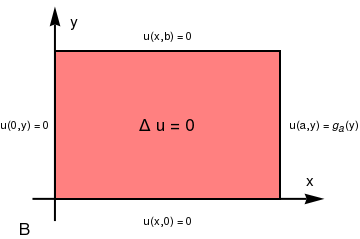
To solve problem B, we proceed in exactly the same as in the previous problem: set \( u(x,y) = X(x)\,Y(y) \) and substitute into the Laplace equation and homogeneous boundary conditions in y. This gives the familiar Sturm--Liouville problem for Y:
\[ Y'' (y) + \lambda\,Y(y) =0 , \qquad Y(0) =0, \quad Y(b) =0. \]
Its solution is well-known:
\[ \lambda_n = \left( \frac{n\pi}{b} \right)^2 , \qquad Y_n (y) = \sin \frac{n\pi y}{b} , \qquad n=1,2,\ldots . \]
Then for X = Xn(x), we get the following differential equation:
\[ X'' (x) - \left( \frac{n\pi}{b} \right)^2 X(x) =0 , \]
which has the general solution
\[ X_n (x) = c_{1n} \cosh \frac{n\pi x}{b} + c_{2n} \sinh \frac{n\pi x}{b} . \]
To satisfy the homogeneous boundary condition at x = 0, we have to set c1n = 0, leaving the another constant c2n arbitrary. The solution of the given Dirichlet problem B for Laplace's equation is assumed to be represented as the sum of all partial nontrivial solutions:
\[ u(x,y) = \sum_{n\ge 1} X_n (x)\, Y_n (y) . \]
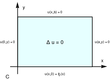
Since each term in the above sum satisfies Laplace's equation and the homogeneous boundary conditions in variables y and x \( u(x,0) = u(x,b) =0 \quad \mbox{and} \quad u(0,y) = 0, \) we know that the sum has the same property (subject to uniform convergence, which is assumed). To satisfy the boundary conditions in variable x, we have
\[ u(0,y) = \sum_{n\ge 1} X_n (0)\, Y_n (y) =0 \qquad\mbox{and} \qquad u(a,y) = \sum_{n\ge 1} X_n (a)\, Y_n (y) = g_a (y) . \]
Therefore, if we set \( X_n (0) =0 , \) which is equivalent to \( c_{1n} =0, \) it will guarantee that the first boundary condition holds. With this in hand, we obtain the general solution:
\[ u(x,y) = \sum_{n\ge 1} X_n (x)\, Y_n (y) = \sum_{n\ge 1} A_n \sinh \frac{n\pi x}{b} \, \sin \frac{n\pi y}{b} , \]
where coefficients An should be chosen so that the identity
\[ u(a,y) = \sum_{n\ge 1} X_n (a)\, Y_n (y) = \sum_{n\ge 1} A_n \sinh \frac{n\pi a}{b} \, \sin \frac{n\pi y}{b} = g_a (y) . \]
is valid. However, this is just Fourier sine series for function g, and its coefficients follow from Euler's formulas:
\[ A_n \sinh \frac{n\pi a}{b} = \frac{2}{b} \int_0^b g_a (y)\, \sin \frac{n\pi y}{b} \,{\text d}y \qquad \Longrightarrow \qquad A_n = \dfrac{2}{b\,\sinh \frac{n\pi a}{b}} \, \int_0^b g_a (y)\, \sin \frac{n\pi y}{b} \,{\text d}y , \qquad n=1,2,3,\ldots . \]

Problem 1CD: We reformulate this problem explicitly: find a solution of Laplace's equation

\[ \Delta u =0 \qquad\mbox{or} \qquad \nabla^2 u =0 , \qquad (x,y) \in (0,a)\times (0,b) , \]
subject to homogeneous boundary conditions in variable x and nonhomogeneous in variable y:

\[ u(0,y) = 0 , \quad u(a,y) = 0, \quad u(x,0) =f_0 (x), \quad u(x,b) = f_b (x). \]
The first step in application of separation of variables consists in extracting an auxiliary problem

\[ \Delta u =0 , \qquad u(0,y) = 0 , \quad u(a,y) = 0, \]
which solution we seek in the form of the product \( u(x,y) = X(x) \, Y(y) . \) Substituting this product into Laplace's equation and homogeneous boundary conditions, we obtain the Sturm--Liouville problem
\[ X'' + \lambda\, X (x) =0, \qquad X(0) =0, \quad X(a) =0 ; \]
and corresponding equation for Y:
\[ Y'' (y) + \lambda\, Y (y) =0. \]
The above Sturm--Liouville problem has a sequence of eigenvalues and eigenfunctions
\[ \lambda_n = \left( \frac{n\pi}{a} \right)^2 , \qquad X_n (x) = \sin \frac{n\pi x}{a} , \qquad n=1,2,3,\ldots . \]
Then the corresponding equation for Y has the general solution in the finite interval \( 0 < y < b : \)
\[ Y_n (y) = a_n \cosh \frac{n\pi y}{a} + b_n \sinh \frac{n\pi y}{a} , \qquad n=1,2,3,\ldots . \]
The superposition principle yields the solution of the given problem C+D:
\[ u(x,y) = \sum_{n\ge 1} X_n (x)\, Y_n (y) = \sum_{n\ge 1} \left[ a_n \cosh \frac{n\pi y}{a} + b_n \sinh \frac{n\pi y}{a} \right] \sin \frac{n\pi x}{a} . \]
Substituting this series solution into nonhomogeneous boundary condition, we obtain the following equations to be held:
\begin{eqnarray*} f_0 (x) &=& u(x,0) = \sum_{n\ge 1} a_n \sin \frac{n\pi x}{a} , \\ f_b (x) &=& u(x,b) = \sum_{n\ge 1} \left[ a_n \cosh \frac{n\pi b}{a} + b_n \sinh \frac{n\pi b}{a} \right] \sin \frac{n\pi x}{a} . \end{eqnarray*}
Since both of then are just sine Fourier expansions of functions f0 and fb, we find their coefficients:
\begin{eqnarray*} a_n (x) &=& \frac{2}{a} \int_0^a f_0 (x) \, \sin \frac{n\pi x}{a} \,{\text d}x , \qquad n=1,2,\ldots ; \\ b_n &=& \frac{2}{a\,\sinh \frac{n\pi b}{a}} \int_0^a f_0 (x) \, \sin \frac{n\pi x}{a} \,{\text d}x - a_n \mbox{coth} \frac{n\pi b}{a} , \qquad n=1,2,\ldots . \end{eqnarray*}

Example: 
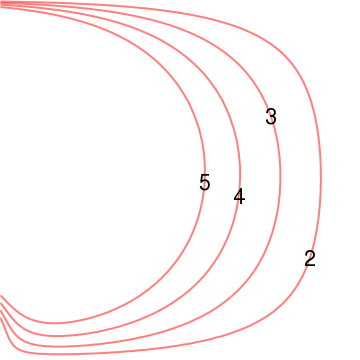
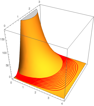
Find the potential inside a cubical box [0,a]×[0,b]×[0,c] with grounded walls, except for the side at z = c which has potential \( \displaystyle V_0 \left[ 1 - \left( \frac{2x}{a} -1 \right)^2 \right] . \) his potential increases from zero at the walls to V0 at x = a/2.

There is no charge inside the box, so the potential satisfies Laplace’s equation

\[ \nabla^2 u =0 \qquad\mbox{or} \qquad \frac{\partial^2 u}{\partial x^2} + \frac{\partial^2 u}{\partial y^2} + \frac{\partial^2 u}{\partial z^2} =0 \]
in a cube with sides a in x, b in y, and c in z with Dirichlet boundary conditions. We try to separate variables by seeking for nontrivial solutions of the form \( u(x,y,z) = X(x)\,Y(y)\,Z(z) . \) Then
\[ X'' Y Z + X Y'' Z = XYZ'' =0 \qquad \Longleftrightarrow \qquad \frac{X''(x)}{X(x)} + \frac{Y''(y)}{Y(y)} + \frac{Z''(z)}{Z(z)} = 0. \]
For the above equation t hold, we must have
\[ \frac{X''(x)}{X(x)} = k_1 , \qquad \frac{Y''(y)}{Y(y)} = k_2 , \qquad \frac{Z''(z)}{Z(z)} = k+3 \qquad\mbox{and} \qquad k_1 + k_2 + k+3 =0. \]
The potential is zero at x = 0 and at x = a, so we need k1 to be negative and equals to \( - \left( \frac{n\pi}{a} \right)^2 . \) Similar argument gives \( k_2 = - \left( \frac{m\pi}{b} \right)^2 , \) and \( Y_m (y) = \sin \frac{m\pi y}{b} . \) Finally,
\[ k_3 = \left( \frac{n\pi}{a} \right)^2 + \left( \frac{m\pi}{b} \right)^2 , \qquad n= 1,2,\ldots , \quad m=1,2,3,\ldots . \]
To make Z equals zero at z = c, the appropriate solution for Z is sine hyperbolic and we have
\[ u(x,y,z) = \sum_{n\ge 1} \sum_{m\ge 1} A_{n,m} \sin \frac{n\pi x}{a} \,\sin \frac{m\pi y}{b} \,\sinh \left( \sqrt{\left( \frac{n\pi}{a} \right)^2 + \left( \frac{m\pi}{b} \right)^2} \, z \right) . \]
Finally we evaluate the potential at z = c:
\[ u(x,y,c) = V_0 \left[ 1 - \left( \frac{2x}{a} -1 \right)^2 \right] = \sum_{n\ge 1} \sum_{m\ge 1} A_{n,m} \sin \frac{n\pi x}{a} \,\sin \frac{m\pi y}{b} \,\sinh \left( \sqrt{\left( \frac{n\pi}{a} \right)^2 + \left( \frac{m\pi}{b} \right)^2} \, c \right) . \]
Following V.A. Steklov, we multiply both sides of the latter by eigenfunctions and integrate the outcome. Using the orthogonality of the sines, we get
\[ \int_0^a {\text d}x\,\sin \frac{n\pi x}{a} \, \int_0^b {\text d}y\,\sin \frac{m\pi y}{b} \, V_0 \left[ 1 - \left( \frac{2x}{a} -1 \right)^2 \right] = \frac{ab}{4}\,A_{n,m} \, \sinh \left( \sqrt{\left( \frac{n}{a} \right)^2 + \left( \frac{m}{b} \right)^2} \, \pi c \right) . \]
With the aid of Mathematica, we evaluate the integral:
Integrate[Sin[m*Pi*y/b],{y,0,b}]
(b - b Cos[m \[Pi]])/(m \[Pi])
Integrate[(1-(2*x/a-1)^2)*Sin[n*Pi*x/a],{x,0,a}]
-((4 a (-2 + 2 Cos[n \[Pi]] + n \[Pi] Sin[n \[Pi]]))/(n^3 \[Pi]^3))
Therefore,
\[ \frac{b}{m\pi} \left[ 1- (-1)^m \right] \frac{8}{n^3 \pi^3} \left[ 1 - (-1)^n \right] V_0 = \frac{ab}{4}\,A_{n,m} \, \sinh \left( \sqrt{\frac{n^2}{a^2} + \frac{m^2}{b^2} } \, \pi c \right) , \]
which allows us to determine the value of An,m:
\[ A_{n,m} = \frac{V_0 32}{\sinh \left( \sqrt{\frac{n^2}{a^2} + \frac{m^2}{b^2} } \, \pi c \right)} \,\frac{1}{m\,n^3 \,\pi^4} \left[ 1- (-1)^m \right] \left[ 1 - (-1)^n \right] , \qquad n,m = 1,2,3,\ldots . \]
Of course, these values are not zeroes only for odd indices. ■

Problem A Dirichlet problem A for Helmholtz equation:

\[ \nabla^2 u(x,y) + k^2 u(x,y) =0, \qquad u(0,y) = g_0 (y) , \quad u(a,y) =0, \quad u(x,0) =0, \quad u(x,b) =0 . \]
We seek its partial nontrivial solutions in the form \( u(x,y) = X(x)\,Y(y) \) that satisfy the homogeneous boundary conditions in y: \( u(x,0) = u(x,b) =0 . \) Upon substitution of the product into the Helmholtz equation, we get
\[ X''\,Y +X\,Y'' + k^2 X\,Y =0 \qquad\mbox{or} \qquad \frac{X''}{X} + \frac{Y''}{Y} + k^2 =0 . \]
Separation of variables yields
\[ \frac{X''}{X} + k^2 = - \frac{Y''}{Y} = \lambda . \]
Therefore, for Y(y) we have the familiar Sturm--Liouville problem
\[ Y'' + \lambda\,Y =0, \qquad Y(0) = Y(b) =0. \]
We know its eigenvalues and corresponding eigenfunctions:
\[ \lambda_n = \left( \frac{n\pi}{b} \right)^2 , \quad Y_n (y) = \sin \frac{n\pi y}{b} , \qquad n=1,2,3,\ldots . \]
For X, we have the differential equation
\[ X'' (x) - \left( \lambda_n - k^2 \right) X(x) =0, \qquad X(a) =0. \]
The general solution of the above differential equation depends on the sign of \( \mu = k^2 - \lambda_n = \left( k - \frac{n\pi}{b} \right) \left( k + \frac{n\pi}{b} \right) . \) Therefore, we have to consider three cases.
  • μ > 0 or kb >nπ. The solution becomes
    \[ X_{n} (x) = \sin \left( \sqrt{k^2 - \lambda_n} (a-x) \right) . \]
  • μ = 0 or kb = nπ. The solution is
    \[ X_{kb/\pi} (x) = a-x . \]
  • μ < 0 or kb <nπ. The solution becomes
    \[ X_{n} (x) = \sinh \left( \sqrt{\lambda_n - k^2} (a-x) \right) . \]
The required solution to Dirichlet problem for Helmholtz equation is the infinite sum of all partial nontrivial solutions:
\[ u(x,y) = \sum_{n\ge 1} c_n \,\frac{X_{n} (x)}{X_n (0)} \,Y_n (y) , \]
where coefficients are determined from the Fourier series
\[ u(0,y) = g_0 (y) = \sum_{n\ge 1} c_n \,Y_n (y) . \]
So we get
\[ c_n = \frac{2}{b} \int_0^b g_0 (y)\, Y_n (y)\,{\text d}y , \qquad n=1,2,\ldots . \]

Dirichlet Boundary Value Problems on Infinite Domains

Example: Consider the Dirichlet problem for Laplace's equation in the semi-strip:
\[ \frac{\partial^2 u}{\partial x^2} + \frac{\partial^2 u}{\partial y^2} = 0, \quad \mbox{inside } -\infty < x < \infty , \ 0 < y < \infty , \qquad u(x,0 ) = f(x) , \]
where f(x) is given. We seek its solution in a class of functions that approach zero at infinity together with their derivatives:
\[ u,\ \frac{\partial u}{\partial x} , \ \frac{\partial u}{\partial y} \ \to \ 0 \quad \mbox{as} \quad \sqrt{x^2 + y^2} \to \infty . \]

Applying the Fourier transformation in variable x, we get

\begin{align*} ℱ\left[ \frac{\partial^2 u}{\partial x^2} \right] (\xi ) &= \int_{-\infty}^{\infty} \frac{\partial^2 u}{\partial x^2} \, e^{{\bf j}x\xi} \,{\text d}x = \left[ \frac{\partial u}{\partial x} \, e^{{\bf j}x\xi} \right]_{x=-\infty}^{x=\infty} - {\bf j}\xi \int_{-\infty}^{\infty} \frac{\partial u}{\partial x} \, e^{{\bf j}x\xi} \,{\text d}x \\ &= 0 - {\bf j}\xi \left\{ \left[ u\,e^{{\bf j}x\xi} \right]_{x=-\infty}^{x=\infty} - {\bf j}\xi \int_{-\infty}^{\infty} u\, e^{{\bf j}x\xi} \,{\text d}x \right\} = -\xi^2 \int_{-\infty}^{\infty} u\, e^{{\bf j}x\xi} \,{\text d}x \\ &= -\xi^2 ℱ\left[ u \right] = -\xi^2 \, \hat{u} . \end{align*}
This transfers the given boundary value problem for PDE into an initial value problem for the ODE:
\[ \frac{{\text d}^2 \hat{u}}{{\text d}y^2}\,\hat{u} - \xi^2 \hat{u} =0, \qquad \hat{u}(0) = \hat{f} = \int_{-\infty}^{\infty} f(x)\,e^{{\bf j}x\xi} \,{\text d}x . \]
Its solution is
\[ \hat{u} (\xi , y) = \hat{f}\,e^{-y|\xi |} \qquad \Longrightarrow \qquad u(x,y) = ℱ^{-1} \left[ \hat{f}\,e^{-y|\xi |} \right] = \frac{1}{2\pi} \int_{-\infty}^{\infty} \hat{f}\,e^{-y|\xi |- {\bf j} x\xi} \,{\text d}\xi = ℱ^{-1} \left[ \hat{f}\, G \right] = f*g , \]
where
\[ g(x,y) = ℱ^{-1} \left[ G(\xi ) \right] = ℱ^{-1} \left[ e^{-y|\xi |} \right] . \]
Therefore,
\begin{align*} g(x,y) &= ℱ^{-1} \left[ G \right] = \frac{1}{2\pi} \int_{-\infty}^{\infty} e^{-y|\xi |- {\bf j} x\xi} \,{\text d}\xi = \frac{1}{2\pi} \int_{-\infty}^0 e^{\xi \left( y-{\bf j}x \right)} \,{\text d}\xi + \frac{1}{2\pi} \int_{0}^{\infty} e^{\xi \left( y+{\bf j}x \right)} \,{\text d}\xi \\ &= \frac{1}{2\pi} \left[ \frac{1}{y - {\bf j}x} + \frac{1}{y + {\bf j}x} \right] , \qquad y> 0, \\ &= \frac{1}{\pi} \,\frac{y}{x^2 + y^2} . \end{align*}
Making convolution with the function g, we obtain the required solution
\[ u(x,y) = f*g = \frac{y}{\pi} \int_{-\infty}^{\infty} \frac{f(s)}{(x-s)^2 + y^2}\,{\text d}s , \qquad y> 0, \]
known as the Poisson formula.


Example B: Consider the Dirichlet problem in the first quarter:
\[ \frac{\partial^2 u}{\partial x^2} + \frac{\partial^2 u}{\partial y^2} =0 \quad (0 < x,y < \infty ), \qquad u(0,y) = f(y), \quad u(x,0) = g(x) , \]
assuming that u tends to zero as \( \displaystyle \sqrt{x^2 + y^2} \to \infty . \)

We solve this boundary value problem with the aid of sine Fourier transform. So we multiply Laplace's equation by sin (kx) and integrate with respect to x from 0 to infinity.

\[ \int_0^{\infty} \frac{\partial^2 u}{\partial x^2}\, \sin (kx) \,{\text d}x + \int_0^{\infty} \frac{\partial^2 u}{\partial y^2} \, \sin (kx) \,{\text d}x = 0. \]
Integration by parts twice yields
\[ \int_0^{\infty} \frac{\partial^2 u}{\partial x^2}\, \sin (kx) \,{\text d}x = \left. \frac{\partial u}{\partial x} \,\sin kx \right\vert_{x=0}^{\infty} - \int_0^{\infty} \frac{\partial u}{\partial x}\, k\,\cos (kx) \,{\text d}x = k\,u(0,y) - k^2 u^S , \]
where
\[ u^S (k,y) = ℱ_s \left[ u(x,y) \right] = \int_0^{\infty} u(x,y)\,\sin kx\,{\text d}x \]
is the sine Fourier transform of function u with respect to x variable. This allows us to rewrite the given partial differential equation as an ordinary differential equation:
\[ \frac{{\text d}^2 u^S}{{\text d} y^2} - k^2 u^S = -k\,f(y) \quad (0 < y < \infty ), \qquad u^S (k,0) = g^S (k) , \]
where
\[ g^S (k) = ℱ_s \left[ g(x) \right] = \int_0^{\infty} g(x)\,\sin kx\,{\text d}x \]
is the sine Fourier transform of the given function g. Solution of the above boundary value problem is
\[ u^S (k,y) = \frac{1}{k}\, \int_0^y \sinh k\left( y- \xi \right) f(\xi )\,{\text d}\xi + g^S \,e^{-ky} . \]
Then we apply the inverse sine Fourier transform
\[ u(x,y) = ℱ^{-1}_s \left[ u^S (k,y) \right] = u_f (x,y) + u_g (x,y) , \]
where
\begin{align*} u_f (x,y) &= ℱ_s^{-1} \left[ \frac{1}{k}\, \int_0^y \sinh k\left( y- \xi \right) f(\xi )\,{\text d}\xi \right] = \frac{2}{\pi} \int_0^{\infty} \frac{\sin (ky)}{k} \,{\text d}k \int_0^y \sinh k\left( y- \xi \right) f(\xi )\,{\text d}\xi \\ u_g (x) &= ℱ_s^{-1} \left[ g^S \,e^{-ky} \right] = g \overset{1}{*} \phi \end{align*}
with
\[ \phi (x) = ℱ^{-1}_s \left[ e^{-ky} \right] = \frac{2}{\pi} \int_0^{\infty} e^{-ky} \,\sin (kx)\,{\text d}k = \frac{2}{\pi} \, \frac{x}{x^2 + y^2} . \]
Assuming[y > 0 && x > 0, Integrate[Exp[-k*y]*Sin[k*x], {k, 0, Infinity}]]
x/(x^2 + y^2)
As we see, the function uf is hard to determined because it is expressed via the double integral. However, function ug is expressed as the special form of convolution:
\[ u_g (x,y) = \frac{1}{\pi} \int_0^{\infty} g(\xi ) \left[ \frac{x}{y^2 + (x-\xi )^2} - \frac{x}{y^2 + (x+\xi )^2} \right] {\text d}\xi . \]
Since variables x and y are symmetrical in our problem, we can use sine Fourier transform with respect to variable y and obtain
\[ u_f (x,y) = \frac{y}{\pi} \int_0^{\infty} f(\xi ) \left[ \frac{1}{x^2 + (y-\xi )^2} - \frac{1}{x^2 + (y+\xi )^2} \right] {\text d}\xi . \]
    ■

Example: 
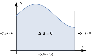
Consider a semi-infinite strip with specified temperature that modeled by the following Dirichlet problem:

\[ \begin{split} u_{xx} + u_{yy} =0 , \qquad 0 < x < a, \quad 0 < y < \infty ; \\ u(0,y) = A, \qquad u(a,y) = B , \qquad 0 < y < \infty ; \\ u(x,0) = f(x) \qquad 0 < x < a, \qquad u(x,y) \,\mapsto \,0 \quad\mbox{as}\quad y \to \infty , \end{split} \]
where A and B are constants. It should be noted that such choice of boundary functions is not realistic because it is impossible to maintain constant temperatures (other than zero) on the boundaries x=0 and x=a because it requires infinite energy supply. In reality, A and B are functions of y decaying with y so they are square integrable (=finite energy).
wave=Plot[3+Sin[0.5*t*Pi], {t,0,3}, Filling ->Axis, PlotRange-> {0,4}];
left = Graphics[ Text[Style["u(0,y) = A"], {-0.5, 1.5}]];
ax = {Arrowheads[Large], Arrow[{{-0.3, 0}, {3.6, 0}}]} ;
ax1 = Graphics[{Thick, Black, ax}] ;
ay = {Arrowheads[Large], Arrow[{{0, -0.3}, {0, 4.2}}]} ;
ay1 = Graphics[{Thick, Black, ay}];
txt1 = Graphics[Text[Style["x", FontSize -> 14], {3.4, 0.35}]];
txt2 = Graphics[Text[Style["y", FontSize -> 14], {0.25, 4.1}]];
right = Graphics[ Text[Style["u(x,b) = B"], {3.5, 1.5}]];
delta = Graphics[ Text[Style["\[CapitalDelta] u = 0", FontSize -> 16], {1.5, 1.5}]];
down = Graphics[ Text[Style[ "u(x,0) = f(x)"], {1.5, -0.3}]];
line = Graphics[ {{Black,Thick},Line[{{3,0},{3,3.4}}]}];

Show[ax1, ay1, wave, txt1, txt2, delta, left, right, down, line, AspectRatio -> 2/3]
Domain for Dirichlet's problem.

We have two options to solve this problem: separation of variables method and sine Fourier transform. We show how both options work, starting with the latter.

We can apply separation of variables only when boundary conditions in one of the variables are homogeneous. Therefore, we represent the required solution as the sum

\[ u(x,y) = w(x,y) + v(x,y) , \]
where w(x,y) is any function that satisfies the Dirichlet boundary condition in variable x:
\[ w(0,y) = A , \qquad w(a,y) =B. \]
So we choose \( \displaystyle w = \frac{x}{a}\,B + \frac{a-x}{a} \,A , \) which obviously satisfies the required boundary conditions in variable x. Then for v, we get a similar Dirichlet problem but with homogeneous boundary conditions in variable x:
\[ \begin{split} v_{xx} + v_{yy} =0 , \qquad 0 < x < a, \quad 0 < y < \infty ; \\ v(0,y) = 0 \qquad v(a,y) = 0 , \qquad 0 < y < \infty ; \\ v(x,0) = f(x) - w(x) \qquad 0 < x < a, \qquad v(x,y) \,\mapsto \,0 \quad\mbox{as}\quad y \to \infty . \end{split} \]
Now we apply separation of variables. We seek partial nontrivial solutions of the Laplace equation Δv=0 that satisfy the homogeneous boundary conditions in variable x, and is represented as a product of two functions
\[ v(x,y) = X(x)\,Y(y) . \]
Substituting this form of solutions into the Laplace equation and boundary conditions in the variable x, we obtain the following differential equation in Y
\[ Y'' (y) - \lambda\,Y(y) =0 , \qquad Y(y) \mapsto 0 \quad\mbox{as} \quad y\to \infty ; \]
and the Sturm--Liouville problem for X:
\[ X'' (x) + \lambda\,X(x) =0 , \qquad X(0) =0, \quad X(a) =0 . \]
Since the latter is a familiar problem, we know its eigenvalues and eigenfunctions:
\[ X_n (x) = \sin \frac{n\pi x}{a} , \qquad \lambda_n = \left( \frac{n\pi}{a} \right)^2 , \quad n=1,2,3,\ldots . \]
Setting λ equals λn, the eigenvalue, we get the problem for Y:
\[ Y'' (y) - \left( \frac{n\pi}{a} \right)^2 Y(y) =0 , \qquad Y(y) \mapsto 0 \quad\mbox{as} \quad y\to \infty . \]
The above problem has a family of solutions
\[ Y_n (y) = c_n e^{-n\pi y/a} , \qquad n=1,2,3,\ldots , \]
depending on a constant multiple cn. Therefore, partial nontrivial solutions will be
\[ v_n (x,y) = X_n (x)\, Y_n (y) = c_n e^{-n\pi y/a} \, \sin \frac{n\pi x}{a} , \qquad n=1,2,3,\ldots . \]
Now we represent the required solutions as a composition of all partial solutions:
\[ v(x,y) = \sum_{n\ge 1} c_n e^{-n\pi y/a} \, \sin \frac{n\pi x}{a} , \]
where coefficients should be chosen to satisfy the boundary condition in variable y:
\[ v(x,0) = \sum_{n\ge 1} c_n \, \sin \frac{n\pi x}{a} = f(x). \]
Therefore,
\[ c_n = \frac{2}{a} \int_0^a \left[ f(x) - w(x) \right] \sin \frac{n\pi x}{a}\,{\text d}x , \qquad n=1,2,3,\ldots . \]

Now we show how to determine the solution using sine Fourier transform. Recall that the sine Fourier transform of a function f define on semi-infinite interval (0, ∞) is

\[ f^s (p) = \int_0^{\infty} f(y)\,\sin (py)\,{\text d}y , \qquad \mbox{with} \qquad f(y) = \frac{2}{\pi} \int_0^{\infty} f^s (p)\,\sin (py)\,{\text d}p . \]
To apply the sine Fourier transform, we need an important identity:
\[ f'' (y) = \frac{2}{\pi} \int_0^{\infty} \left[ p\,f(0) - p^2 f^s (p) \right] \sin py\,{\text d}p . \]
So we multiply the Laplace equation by sin(px) and integrate the result with respect to y. This yields
\[ \frac{{\text d} u^s}{{\text d}x^2} - p^2 u^s (x,p) + p\,f(x) =0 , \qquad 0<x<a, \qquad u^s (0,p) = A^s (p) , \quad u^s (a,p) = B^s (p) , \]
where
\[ A^s (p) = \int_0^{\infty} A(y)\,\sin (py)\,{\text d}y , \qquad B^s (p) = \int_0^{\infty} B(y)\,\sin (py)\,{\text d}y \]
are sine Fourier transforms of functions A(y) and B(y), respectively. I believe that Mathematica knows how to solve the corresponding homogeneous boundary value problem and how to determine the Green function.
DSolve[{u''[x] -p^2 *u[x] ==0, u[0]==A, u[a]==B}, u, x ]
{{u -> Function[{x}, ( E^(-p x) (-B E^(a p) + A E^(2 a p) - A E^(2 p x) + B E^(a p + 2 p x)))/(-1 + E^(2 a p))]}}
DSolve[{u''[x] -p^2 *u[x] ==0, u[0]==0, u[a]==1}, u[x], x ]
{{u[x] -> (E^(a p - p x) (-1 + E^(2 p x)))/(-1 + E^(2 a p))}}
Therefore, the sine Fourier transform of the unknown solutions is
\[ u^s (x,p) = \int_)^x \frac{\sinh p(x-\xi )}{\sinh pa} \,f(\xi )\,{\text d}\xi + A^s \,\frac{\sinh p(a-x)}{\sinh ap} + B^s \,\frac{\sinh ax}{\sinh ap} \]
Then the required function will be obtained by applying the inverse sine Fourier transform:
\[ u(x,y) = \frac{2}{\pi} \int_0^{\infty} u^s (x,p) \,\sin (yp)\,{\text d}p . \]


Return to Mathematica page
Return to the main page (APMA0340)
Return to the Part 1 Matrix Algebra
Return to the Part 2 Linear Systems of Ordinary Differential Equations
Return to the Part 3 Non-linear Systems of Ordinary Differential Equations
Return to the Part 4 Numerical Methods
Return to the Part 5 Fourier Series
Return to the Part 6 Partial Differential Equations
Return to the Part 7 Special Functions