Preface


This tutorial was made solely for the purpose of education and it was designed for students taking Applied Math 0340. It is primarily for students who have some experience using Mathematica. If you have never used Mathematica before and would like to learn more of the basics for this computer algebra system, it is strongly recommended looking at the APMA 0330 tutorial. As a friendly reminder, don't forget to clear variables in use and/or the kernel. The Mathematica commands in this tutorial are all written in bold black font, while Mathematica output is in normal font.

Finally, you can copy and paste all commands into your Mathematica notebook, change the parameters, and run them because the tutorial is under the terms of the GNU General Public License (GPL). You, as the user, are free to use the scripts for your needs to learn the Mathematica program, and have the right to distribute this tutorial and refer to this tutorial as long as this tutorial is accredited appropriately. The tutorial accompanies the textbook Applied Differential Equations. The Primary Course by Vladimir Dobrushkin, CRC Press, 2015; http://www.crcpress.com/product/isbn/9781439851043

Return to computing page for the first course APMA0330
Return to computing page for the second course APMA0340
Return to Mathematica tutorial for the first course APMA0330
Return to Mathematica tutorial for the second course APMA0340
Return to the main page for the first course APMA0330
Return to the main page for the second course APMA0340
Return to Part VI of the course APMA0340
Introduction to Linear Algebra with Mathematica

Numerical Solutions to Wave Equation


Consider the wave equation

\[ \square_c u =0 \qquad\mbox{or} \qquad \frac{\partial^2 u}{\partial t^2} = c^2 \frac{\partial^2 u}{\partial x^2} , \qquad 0 < x < \ell , \quad 0 < t < b, \]
subject to the boundary conditions:
\[ u(0,t) =0 \qquad u(\ell , t) = 0 , \qquad 0 < t < b, \]
and the initial conditions:
\[ u(x,0) = f(x) \qquad u_t (x , 0) \equiv \left. \frac{\partial u}{\partial t} \right\vert_{t=0} = g(x) , \qquad 0 < x < \ell . \]
Here f(x) and g(x) are specified functions of spacial variable x and c is the speed of the wave.

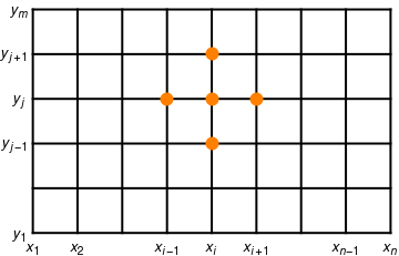
We partition the rectangle \( R = \left\{ (x,t)\, : \, 0 \le x \le \ell , \ 0 \le t \le b \right\} \) into a grid consisting of n-1 by m-1 rectangles with sides \( \Delta x = h \) and Δt = k, as shown in Figure.

The grid used for solving wave equation
Start at the bottom row, where \( t= t_1 =0 \) and the solution is known to be \( u(x_i , t_1 ) = u(x_i , 0 ) = f(x_i ) . \) We shall use a difference-equation method to compute approximations
\[ \left\{ u_{i,j} \, : \, i =1,2,\ldots , n \right\} \quad \mbox{in successive rows} \qquad \mbox{for}\quad j=2,3,\ldots , m . \]
The true solution value at the mesh points is \( u(x_i , t_j ) . \)

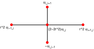
The central-difference formulas for approximating utt(x,t) and uxx(x,t) are

\[ \begin{split} u_{tt} (x,t) &= \frac{u(x,t+k) -2u(x,t) + u(x,t-k)}{k^2} + O\left( k^2 \right) , \\ u_{xx} (x,t) &= \frac{u(x+h, t) -2u(x,t) + u(x-h,t)}{h^2} + O\left( h^2 \right) . \end{split} \]
The grid spacing is uniform in every row: \( x_{i+1} = x_i +h \) (and \( x_{i-1} = x_i -h \) ); and it is uniform in every column: \( t_{j+1} = t_j +k \) (and \( t_{j-1} = t_j -h \) ). Next, we drop the terms O(h2) and O(k2) and use approximation \( u_{i,j} \) for \( u(x_i , t_j ) , \) which produces the difference equation
\[ \frac{u_{i,j+1} -2\,u_{i,j} + u_{i,j-1}}{k^2} = c^2 \frac{u_{i+1,j} -2\,u_{i,j} + u_{i-1,j}}{h^2} . \]
For convenience, the abbreviation t = ck/h is introduced, and the above equation is reduced to
\[ u_{i,j+1} - 2\,u_{i,j} + u_{i,j-1} = r^2 \left( u_{i+1,j} - 2\,u_{i,j} + u_{i-1,j} \right) . \]
The above equation is utilized to determine the values in the row j+1 across the grid, assuming that approximations at both rows j and j-1 are known:
\[ u_{i,j+1} = \left( 2 - 2r^2 \right) u_{i,j} + r^2 \left( u_{i+1,j} + u_{i-1,j} \right) - u_{i,j-1} , \]
for i = 2,3,...,n-1. The computational stencil is shown below.
l0 = Graphics[{Thick, Line[{{-4, 0}, {4, 0}}]}];
l1 = Graphics[{Thick, Line[{{0, -2}, {0, 2}}]}];
d0 = Graphics[{Red, Disk[{0, 0}, 0.15]}];
d1 = Graphics[{Red, Disk[{4, 0}, 0.15]}];
d2 = Graphics[{Red, Disk[{-4, 0}, 0.15]}];
d3 = Graphics[{Red, Disk[{0, 2}, 0.15]}];
d4 = Graphics[{Red, Disk[{0, -2}, 0.15]}];
r1 = Graphics[ Text[Style["(2-2r^2)\!\(\*SubscriptBox[\(u\), \(i,j\)]\)", Medium], {1.1, -0.5}]];
r2 = Graphics[Text[ Style["r^2 \!\(\*SubscriptBox[\(u\), \(i+1,j\)]\)", Medium], {4.4, -0.5}]];
r3 = Graphics[Text[ Style["r^2 \!\(\*SubscriptBox[\(u\), \(i-1,j\)]\)", Medium], {-4.5, -0.3}]];
r4 = Graphics[Text[ Style["\!\(\*SubscriptBox[\(u\), \(i,j+1\)]\)", Medium], {0, 2.5}]];
r5 = Graphics[Text[ Style["-\!\(\*SubscriptBox[\(u\), \(i,j-1\)]\)", Medium], {0.3, -2.4}]];
Show[l0, l1, d0, d1, d2, d3, d4, r1, r2, r3, r4, r5]
The wave equation stencil
Caution must be taken when using the above explicit difference formula. If the error made at one stage of the calculations is eventually dampened out, the method will be stable. To guarantee stability in this formula, it is necessary to employ the CFL condition r = ck/h ≤ 1. There are known other schemes, called implicit methods, that are more complicated to implement, but do not have stability restriction for r.

Two starting rows of values corresponding to j = 1 and j = 2 must be supplied in order to use the explicit recurrence formula. Since the second row is not usually given, the boundary function g(x) is used to help produce starting approximations in the second row. Fix x = xi at the boundary and apply Taylor's formula of order 1 for expanding u(x,t) about (xi, 0). The value at this point satisfies

\[ u(x_i , k) = u(x,0) + u_t (x_i , 0)\,k + O\left( k^2 \right) . \]
Using the given identities \( u(x_i , 0) = f(x_i ) = f_i \) and \( u_t (x_i ,0) = g(x_i ) = g_i , \) we derive the formula for computing the numerical approximations in the second row:
\[ u_{i,2} = _i + k\,g_i \qquad\mbox{for } i=2,3,\ldots , n-1. \]
As a rule, \( u(x_i , t_2 ) \ne u_{i,2} , \) and such errors introduced by the above approximation formula will propagate throughout the grid and will not be dampened out when the explicit scheme is implemented. Hence, it is prudent to use a very small step size for k so that the values for ui,2 do not contain a large amount of truncation error.

Often, the boundary function f(x) has a second derivative over the interval. In this case, we have \( u_{xx} (x,0) = f'' (x) , \) and it is beneficial to use the Taylor formula of order 2 to help construct the second row. To do this, we go back to the wave equation and use the relationship between the second order partial derivatives to obtain

\[ u_{tt} (x_i , 0) = c^2 u_{xx} (x_i , 0) = c^2 f'' (x_i ) = c^2 \frac{f_{i+1} - 2\, f_i + f_{i-1}}{h^2} + O \left( h^2 \right) . \]
Using Taylor's formula of order 2
\[ u(x,k) = u(x,0) + u_t (x,0)\,k + \frac{1}{2}\, u_{tt} (x,0) \, k^2 + O \left( k^3 \right) , \]
we obtain
\[ u(x_i , k) = f_i + k\, g_i + \frac{c^2 k^2}{2\,h^2} \left( f_{i+1} -2\, f_i + f_{i-1} \right) + O \left( h^2 \right) O \left( k^2 \right) + O \left( k^3 \right) . \]
Using notation r = ck/h, the above formula can be simplified:
\[ u_{i,2} = \left( 1 - r^2 \right) f_i + k\, g_i + \frac{r^2}{2} \left( f_{i+1} + f_{i-1} \right) \]
for i = 2,3,...,n-1.


II. Two Exact Rows given


the accuracy of the numerical approximations depends on the truncation errors in the formulas used to convert the partial differential equation into a difference equation. Although it is unlikely to know values of the exact solution for the second row of the grid, if such knowledge were available, using the increment k = ch along the t-axis will generate an exact solution at all the other points throughout the grid.

Theorem: Assume that the two rows of values ui,1 = u(xi,0) and ui,2 = u(xi,k), for i = 1,2,...,n, are the exact solutions to the wave equation. If the step size k=h/c is chosen along the t-axis, then r=1 and we have
\[ u_{i,j+1} = u_{i+1,j} + u_{i-1,j} - u_{i,j-1} . \]
Furthermore, the finite-difference solutions produced by the above formula throughout the grid are exact solution values to the differential equation (neglecting computer round-off error). ■

Note: Theorem does not guarantee that the numerical solutions are exact when numerical calculations based on

\[ u_{i,2} = \left( 1 - r^2 \right) f_i + k\, g_i + \frac{r^2}{2} \left( f_{i+1} + f_{i-1} \right) \]
are used to construct approximations ui,2 in the second row. Indeed, truncation error will be introduced if ui,2u(xi,k) for some i, where 1 ≤ in.This is why we endeavor to obtain the best possible values for the second row by using the second order Taylor approximations in the above equation.

Program (Finite-difference method for the wave equation): to approximate the solution of \( u_{tt} = c^2 u_{xx} \) over \( R = \{\,(x,t) \,:\, 0 \le x \le \ell , \ 0 \le t \le b \) with u(x,0) = f(x), ut(x,0) = g(x), for 0 ≤ x ≤ ℓ, and u(0,t) = 0, u(ℓ,t) = 0, for 0 ≤ tb.


function U=wave(f,g,a,b,c,n,m)
% Input  -- f=u(x,0) as a string 'f'
%        -- g=ut(x,0) as a string 'g' 
%        -- a and b right end points of [0,a] and [0,b]
%        -- c=the speed constant in wave equation
%        -- n and m number of grid points over [0,a] and [0,b] 
% Output -- U solution matrix; 
% Initialize parameters and U
h=a/(n-1);
k=b/(m-1);
r=c*k/h;
r2=r^2; 
r22=r^2/2;
s1=1-r^2;
s2=2-2*r^2;
U=zeros(n,m);

% Compute first and second rows
for i=2:n-1
    U(i,1)=feval(f,h*(i-1));
    U(i,2)=s1*feval(f,h*(i-1))+k*feval(g,h*(i-1))+r22*(feval(f,h*i) + feval(f,h*(i-2)));
end

% Compute remaining rows of U 
for j=3:m,
    for i=2:(n-1),
        U(i,j) = s2*U(i,j-1)+r2*(U(i-1,j-1)+U(i+1,j-1))-u(i,j-2);
    end
end 

U=U'; 

Example: Consider the initial boundary value problem modeling a vibrating string:

\[ u_{tt} (x,t) = 9\,u_{xx} (x,t) \qquad \mox{for } 0< x < 2 \quad\mbox{and}\quad 0 < t < 0.5, \]
with the boundary conditions
\[ u(0,t) =0 \qquad\mbox{and}\qquad u(2,t) =0 \qquad\mbox{for } 0 \le t \le 0.5, \]
and the initial conditions
\[ u(x,0) =f(x) 2\,\sin (\pi x) - 3\,\sin (3\pi x) \qquad\mbox{and}\qquad u_t (x,0) =0 \qquad\mbox{for } 0 \le x \le 2. \]
For convenience, we choose h = 0.1 and k = 0.05. Since c = 3, this yields r = ck/h = 1.5. Because the initial velocity is zero, the second row becomes
\[ u_{i,2} = \frac{1}{2}\left( f_{i-1} + f_{i+1} \right) \qquad\mbox{for } i=2,3,\ldots , 9. \]
Fourth order approximation of the partial derivative \frac{\lartial^2 f}{\partial x \partial y} using Richardson interpolation.
lumfxy[f_, {x_, y_}, {dx_, dy_}] := 1/(144 dx dy)*(f[x - 2 dx, y - 2 dy] - f[x - 2 dx, y + 2 dy] - f[x + 2 dx, y - 2 dy] + f[x + 2 dx, y + 2 dy]) + 1/(18 dx dy) * (f[x - 2 dx, y + dy] - f[x - 2 dx, y - dy] - f[x + 2 dx, y + dy] + f[x + 2 dx, y - dy] + f[x + dx, y - 2 dy] - f[x + dx, y + 2 dy] - f[x - dx, y - 2 dy] + f[x - dx, y + 2 dy]) + 4/(9 dx dy)* (f[x + dx, y + dy] - f[x + dx, y - dy] - f[x - dx, y + dy] + f[x - dx, y - dy])
In[42]:= f[x_, y_] = Sin[x^3 + y^2];
Df[x_, y_] = D[f[x, y], x, y]; numfxy[f, {1.2, 2.1}, {0.1, 0.1}]
Out[44]= 2.53166
In[45]:= Df[1.2, 2.1]
Out[45]= 2.625
In[57]:= data2der = Table[{10.^(-i), Df[1.2, 2.1] - numfxy[f, {1.2, 2.1}, {10^(-i), 10^(-i)}]}, {i, 1, 10}]; TableForm[N[ data2der, 10], TableHeadings -> {None, {"h in x,y", "fxy - fxyapprox"}}]
Out[58]//TableForm= h in x,y fxy - fxyapprox 0.1 0.0933346 0.01 9.17337 ´ 10-6 0.001 9.06194 ´ 10-10 0.0001 -4.1087 ´ 10-9 0.00001 4.36954 ´ 10-7 1. ´ 10-6 0.000294606 . ´ 10-7 0.000148889 1. ´ 10-8 -0.0272019 1. ´ 10-9 -5.27763 1. ´


  1. Abdulkadir, Y. (2015) Comparison of Finite Difference Schemes for the Wave Equation Based on Dispersion. Journal of Applied Mathematics and Physics, 3, 1544-1562. doi: 10.4236/jamp.2015.311179.
  2. Bilbao, S. and Smith, J., Finite Difference Schemes and Digital Waveguide Networks for the Wave Equation: Stability, Passivity, and Numerical Dispersion, IEEE Transactions on Speech and Audio Processing, 2003, Vol. 11, No. 3, pp. 255-266.
  3. Dong, S., Finite Difference Methods for the Hyperbolic Wave Partial Differential Equations
  4. Grigoryan, V., Finite differences for the wave equation
  5. Langtangen, H.P., Finite difference methods for wave motion
  6. Lie, K.-A., The Wave Equation in 1D and 2D
  7. Anthony Peirce, Solving the Heat, Laplace and Wave equations using finite difference methods


Return to Mathematica page

Return to the main page (APMA0340)
Return to the Part 1 Matrix Algebra
Return to the Part 2 Linear Systems of Ordinary Differential Equations
Return to the Part 3 Non-linear Systems of Ordinary Differential Equations
Return to the Part 4 Numerical Methods
Return to the Part 5 Fourier Series
Return to the Part 6 Partial Differential Equations
Return to the Part 7 Special Functions