Return to computing page for the first course APMA0330
Return to computing page for the second course APMA0340
Return to Mathematica tutorial for the first course APMA0330
Return to Mathematica tutorial for the second course APMA0340
Return to the main page for the first course APMA0330
Return to the main page for the second course APMA0340
Return to Part III of the course APMA0340
Introduction to Linear Algebra with Mathematica
The Lyapunov second method was discovered by Alexander Lyapunov in 1892. It is also referred to as the direct method because no knowledge of the solution of the system of autonomous equations is required:
where overdot stands for the derivative with respect to time variable t, \( \dot{\bf x} = {\text d}{\bf x}/{\text d}t . \) The vector x(t) defins the point in an n-dimensional state space for every t.
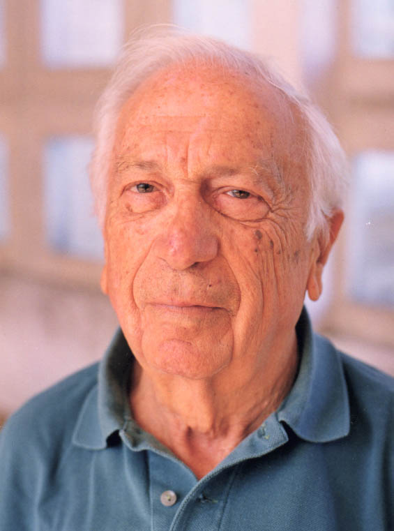
Alexander M. Lyapunov (1857--1918), a
student of P.Chebyshev at St. Petersburg
(Russia), taught at the
University of Kharkov from
1885 to 1901, when he became an academician in applied mathematics at the St. Petersburg Academy of
Science. His surname is variously romanized as Ljapunov, Liapunov, Liapounoff or Ljapunow. In 1917 he
joined his brother's location in Odessa because of his wife's frail health. On day of his wife's death,
Alexander shoot himself with a revolver. Three days later he passed away.
✶
Preliminary terminology
Application of the direct method of A.Lyapunov to the autonomous system of differential equations \eqref{EqLyapunov.1} is based on utilization of a smooth function V(x) that possesses some properties.
The function V : ℝn → ℝ is called positive definite in S⊂ℝn, with respect to x✶, if V has continuous partials, V(x✶) = 0, and V(x) > 0 for all x in S, where x ≠ x✶.
The function V : ℝn → ℝ is called positive semi-definite in S⊂ℝn, with respect to x✶, if V has continuous partials, V(x✶) = 0, and V(x) ≥ 0 for all x in S, where x ≠ x✶.
Similarly, a function V(x) is called negative definite/negative semi-definite if −V(x) is positive definite/positive semi-definite.
Without any loss of generocity, we can assume that the isolated critical point for the vector equation \eqref{EqLyapunov.1} is the origin. A particular example of positive (or negative) definite functions constitute quadratic functions that can written in the form
A real-valued matrix A is called positive definite/positive semi-definite if all its eigenvalues are positive/not negative. Correspondingly, we call matrix B negative definite if −B is positive definite (so all eigenvalues of B are negative real numbers).
Note that our definition is slightly different that is used in mathematics---it is additionally required for matrix P to be self-adjoint (P = P✶). In case of real-valued matrices, the condition becomes P = PT, so matrix must be symmetric. The reason why mathematicians impose symemtry on matrix A is that the inegality
holds for these matrices. When matrix is not symmetric, but has positive eigenvalues, it may satisfy inequality \eqref{EqLyapunov.3} or may not. We relax condition of self-adjointy to be consistent with future applications (Sturm--Liouville problems).
Theorem 1:
Let V(x) = xTPx, where P is a symmetric real-valued matrix, P = PT. Then V(x) is positive definite if and only if all eigenvalues of P are positive. Correspondingly, V(x) is positive semi-definite if and only if all eigenvalues of P are non-negative.
In order to apply Theorem 1 to an arbitrary matrix, we need to symmetrize the given matrix first:
Hence, the given 2×2 matrix does not generate a positive quadratic form.
■
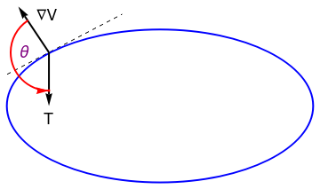
If x(t) is a solution curve of the autonomous equation \eqref{EqLyapunov.1}, then V(x(t)) represents the corresponding values of V along the trajectory. If we want to determine whether this function V(x(t)) increading or decreasing, we need to evaluate the derivative
where
\[
\nabla V = \left[ \frac{\partial V}{\partial x_1} \ \frac{\partial V}{\partial x_2} \ \cdots \ \frac{\partial V}{\partial x_n} \right]
\]
is the gradient of V. The vector \( {\bf T} = \dot{\bf x}(t) \) is the tangent vector to the trajectory.
The derivative \eqref{EqLyapunov.4} is called the derivative of function V(x) with respect to solution of the differential equation dx/dt = f(x) or the Lyapunov derivative.
Using the chain rule, we compute the derivative of V(x(t)):
\[
\dot{V({\bf x})} = \frac{\partial V}{\partial x_1} \cdot \dot{x}_1 + \cdots + \frac{\partial V}{\partial x_n} \cdot \dot{x}_n = \nabla V \cdot \dot{\bf x} = \nabla V \cdot {\bf f} .
\]
V=xTPx, where P=PT, is positive definite if and only if all eigenvalues of P are positiv
V=xTPx, where P=PT, is positive semi-definite if and only if all eigenvalues of P are non-negative
Example
\[
{\bf P} = \begin{bmatrix} 2&-8 \\ 0&\phantom{-}3 \end{bmatrix}
\]
Theorem 2 (Lyapunov):
The real matrix A is asymptotically stable, that is, all eigenvalues of A have negative real parts if and only if for any P, the solution Q of the continuous matrix Lyapunov equation
\[
{\bf A}^{\mathrm T} {\bf P} + {\bf P}\,{\bf A} = -{\bf Q}
\]
is (symmetric) positive definite.
To use the Lyapunov theorem, select an arbitrary symmetric positive definite Q, for example, an identity matrix, I. Then solve the Lyapunov equation for symmetric matrix P = PT.
If P is positive definite, the matrix A generates a positive definite quadratic form V(x) = xTPx, so A is asymptotically stable.
If P is not positive definite, then A is not not a positive definite (not asymptotically stable).
Example
Motovated example
Direct Method
If the origin is asymptotically stable, we seek for a smooth function that V(x) that
provides a unique minimum with respect to all other points in some neighborhood of the equilibrium of
interest. Along any trajectory of the system, the value of V never increases
In order for V(x(t)) not to increase, we require \( \dot{V({\bf x}(t))} \le 0 . \)
Alexander Lyapunov
Theorem (Lyapunov):
Let x* be a fixed point for the vector differential equation
\[
\dot{\bf x} = {\bf f}\left( {\bf x} \right)
\]
and V(x, y) be a differentiable function defined on some
neighborhood W of x* such that
V(x*) = 0 and V(x) > 0 if x
≠ x*;
\( \dot{V} ({\bf x}) \le 0 \) in W ∖
{ x* }.
The the critical point is stable. If in addition, \( \dot{V} ({\bf x}) < 0 \) in W ∖
{ x* }, then the critical point is asymptotically stable.
▣
Lyapunov second method on the plane
If a trajectory is converging to xe=0, it should be possible to find a nested set of closed curves V(x1,x2)=c, c≥0, such that decreasing values of c yield level curves shrinking in on the equilibrium state xe=0
where dot stands for the derivative with respect to time variable t.
The function f(t) is usually called input and
x(t) the response.
It is usually important that x(t) remains bounded for all
t≥0. To this end, we usually require q(x) ≥ 0 for
x≥0, q(x) < 0 for x<0 and
|q(x)| > &delta for all x large
(mechanically speaking, we want q to be a restoring force). Further we
require \( p \left( x, \dot{x} \right) < 0 \)
(i.e., we want damping). If f(t) = 0 for t > 0
(i.e., if the system is undriven) these conditions by themselves are sufficient
to prevent x(t) and its derivative from becoming unbounded as
t ⟼ ∞.
Theorem:
Suppose
p: ℝ² → ℝ is a continuous function with
p(u,v) ≥ 0 for all u,v ∈ ℝ;
q: ℝ → ℝ is a continuous function with
uq(u) ≥ 0 for all u ∈ ℝ and
\( \int_0^y q(u)\,{\text d}u \to \infty \quad \mbox{as} \quad |y| \to \infty . \)
Then, if x: ℝ → ℝ is twice differentiable and
satisfies \( \ddot{x} + p\left( x, \dot{x} \right) \dot{x} + q(x) = 0, \) then there exists a positive constant K (depending
only on the initial displacement and initial velocity) such that
\( |x(t)|, \ |\dot{x}(t)| \le K , \) for all
t≥0.
▣
Its proof is based on the usage of the Lyapunov function
Example 1:
Consider the motion of a particle of mass m attached to a spring of
stiffness \( k \left( x + x^3 \right) , \) where
x is displacement from the equilibrium position. The differential
equation governing the system is
\[
m\,\ddot{x} + k \left( x + x^3 \right) = 0 \qquad \Longleftrightarrow \qquad
\ddot{x} + x + \varepsilon\, x^3 = 0
\]
upon appropriate change the dependent variable. Transferring the second order
equation into a system of first order equations, we get
\[
\begin{split}
\dot{x} &= y , \\
\dot{y} &= - \frac{k}{m} \left( x + x^3 \right) .
\end{split}
\]
The associated total energy of the spring system becomes
This function is also a Lyapunov function for the system because E(0,0)
= 0 at the unique equilibrium solution (x, y) = (0,0) and
E(x, y) > 0 for (x, y) ≠ (0,0). Moreover, the
derivative of the Lyapunov function with respect to the system of equations is
If we choose β sufficiently small, V remains positive definite and its derivative is strictly negative for all (x, y) ≠ (0,0). Hence, the origin is globally asymptotically stable for &akpha; > 0.
■
Example 2:
■
Example 3:
José Luis Massera
We present an example credited to the Uruguayan dissident and mathematician José Luis Massera (1915--2002).
Therefore, V(x, t) is a (positive) Lyapunov function for the given differential equation with negative derivative. However, the origin is not asymptotically stable.
■
Guckenheimer, J. and Holmes, P., Nonlinear Oscillations, Dynamical Systems, and Bifurcations of Vector Fields, Springer-Verlag, New York, 2002; https://doi.org/10.1007/978-1-4612-1140-2
Return to Mathematica page
Return to the main page (APMA0340)
Return to the Part 1 Matrix Algebra
Return to the Part 2 Linear Systems of Ordinary Differential Equations
Return to the Part 3 Non-linear Systems of Ordinary Differential Equations
Return to the Part 4 Numerical Methods
Return to the Part 5 Fourier Series
Return to the Part 6 Partial Differential Equations
Return to the Part 7 Special Functions