Preface


This section is about constant coefficient linear vector differential equations.

Return to computing page for the first course APMA0330
Return to computing page for the second course APMA0340
Return to Mathematica tutorial for the first course APMA0330
Return to Mathematica tutorial for the second course APMA0340
Return to the main page for the first course APMA0330
Return to the main page for the second course APMA0340
Return to Part II of the course APMA0340
Introduction to Linear Algebra with Mathematica

Constant Coefficient Systems of Ordinary Differential Equations


In what follows, we use Newton's notation for the derivative with respect to time variable: \( \dot{y} = {\text d}y/{\text d}t . \) Consider a homogeneous systems of linear differential equations with constant coefficients:

\[ \begin{split} \dot{y}_1 &= a_{11} y_1 + a_{12} y_2 + \cdots + a_{1n} y_n , \\ \dot{y}_2 &= a_{21} y_1 + a_{22} y_2 + \cdots + a_{2n} y_n , \\ \vdots & \qquad \vdots \\ \dot{y}_n &= a_{n1} y_1 + a_{n2} y_2 + \cdots + a_{nn} y_n , \\ \end{split} \]
which we rewrite in compact vector form
\begin{equation} \label{EqConstant.1} \dot{\bf y} (t) = {\bf A} \,{\bf y} (t) \qquad \mbox{or} \qquad \frac{{\text d}{\bf y}}{{\text d} t} = {\bf A} \,{\bf y} (t), \end{equation}
where A is the constant n-by-n matrix of coefficients and y is the n-dimensional column vector of unknown functions:
\[ {\bf A} = \begin{bmatrix} a_{11} & a_{12} & \cdots & a_{1n} \\ a_{21} & a_{22} & \cdots & a_{2n} \\ \vdots & \vdots & \ddots & \vdots \\ a_{n1} & a_{n2} & \cdots & a_{nn} \end{bmatrix} , \qquad {\bf y} (t) = \begin{bmatrix} y_1 \\ y_2 \\ \vdots \\ y_n \end{bmatrix} . \]
A solution y(t) to system of ODEs \eqref{EqConstant.1} is a point in the n-dimentional space ℝn for every t; it is called the state of the system at time t. As t varies, the point y(t) moves along a curve in the space ℝn. This solution curve is called a trajectory, or streamline, or orbit, or phase curve, for the system \eqref{EqConstant.1}.
Since a constant matrix A is is obviously continuous on any interval, all solutions to Eq.\eqref{EqConstant.1} are defined on (−∞, ∞). Therefore, when we speak of solutions to the vector differential equation with constant coefficients \eqref{EqConstant.1}, we consider solutions on the whole real axis. Correspondingly, when we discuss behavior of the solution when t → ∞, we mean either of the limits: t → −∞ or t → +∞. Usually, we will specify what limit we consider because variable t is associated with time.
We refer to a constant solution \( {\bf y}(t) = {\bf y}^{\ast} \) of a linear system of equations as an equilibrium if \( {\text d}{\bf y}/{\text d}t = 0. \) Such a constant solution is also called a critical point or stationary point of the system. An equilibrium solution is isolated if there is a neighborhood to the critical point that does not contain any other critical point.
Recall that a neighborhood is any set of points containing the point or subset of interest inside some open set. For example, a neighborhood containing the origin in one dimension could be [-0.1,1], as it contains the point 0 inside the open symmetric interval (-0.1, 0.1). But [0, 1] is not a neighborhood of the origin as it does not contain any open interval centered at zero. In a two-dimensional space, a neighborhood of the origi could be any set containing an open circle with radius epsilon (x² + y² < ε²), which is centered about the origin.

If matrix A is invertible (detA ≠ 0), then 0 is the only stationary point of the system \eqref{EqConstant.1}. Otherwise, the system has a subspace of equilibrium solutions spanned on the null space of matrix A.

Along with the initial value problem, it is convenient to consider the matrix differential equation for n×n matrix Φ(t):

\[ \frac{\text d}{{\text d}t} {\bf \Phi}(t) = {\bf A}\,{\bf \Phi}(t) . \]
because each of its columns is a solution of the vector equation \eqref{EqConstant.1}.
Any nonsingular solution of the matrix differential equation \( \dot{\bf \Phi} = {\bf A}\,{\bf \Phi}, \quad \det{\bf \Phi}(t) \ne 0, \) is called the fundamental matrix for the vector differential equation \( \dot{\bf y} = {\bf A}\,{\bf y} . \) .
If n×n matrix A is diagonalizable, then it has n linearly independent eigenvectors x1, x2, …, xn, corresponding to eigenvalues λ1, λ2, …, λn, which are not necessarily distinct. In this case the fundamental matrix can be written explicitly:
\[ {\bf X}(t) = \left[ {\bf x}_1 e^{\lambda_1 t} \ {\bf x}_2 e^{\lambda_1 t} \ \cdots \ {\bf x}_n e^{\lambda_n t} \right] , \]
placing every eigenvector with the corresponding exponential multiple side by side. Of course, a fundamental matrix is not unique and its determinant, called the Wronskian, is never zero
\[ W(t) = \det{\bf X}(t) = \det \left[ {\bf x}_1 e^{\lambda_1 t} \ {\bf x}_2 e^{\lambda_1 t} \ \cdots \ {\bf x}_n e^{\lambda_n t} \right] = \mbox{constant} \cdot \exp \left\{ \mbox{tr}\left( {\bf A} \right) t \right\} . \]
Any two fundamental matrices X(t) and Y(t), corresponding to the same matrix A, are constant multip[les of each other
\begin{equation} \label{EqConstant.2} {\bf X}(t) = {\bf Y}(t)\,{\bf C} , \qquad \det {\bf C} \ne 0. \end{equation}

A particular interest exhibits the fundamental matrix solution, called the propagator, that satisfies the specific initial condition

\begin{equation} \label{EqConstant.3} \frac{{\text d} }{{\text d} t}\,{\bf \Phi} = {\bf A} \,{\bf \Phi} (t), \qquad {\bf \Phi} (0) = {\bf I} , \end{equation}
where I is the identity n-by-n matrix. We showed previously using Picard's iteration that the matrix initial value problem \( \dot{\bf \Phi} = {\bf A}\,{\bf \Phi}, \quad {\bf \Phi}(0) = {\bf I} \) has a unique solution that is expresented by a convergent power series for any square matrix A:
\begin{equation} \label{EqConstant.4} {\bf \Phi}(t) = {\bf I} + {\bf A}t + {\bf A}^2 \frac{t^2}{2} + \cdots = \sum_{n\ge 0} {\bf A}^n \frac{t^n}{n!} . \end{equation}
It is natural to denote this series solution by \( {\bf \Phi} (t) = e^{{\bf A}t} \) because this function satisfies the following relations.
Theorem 1: Let A be an n×n matrix with constant entries (real or complex). Then the exponential matrix \eqref{EqConstant.4} is the unique solution of the matrix initial value problem \eqref{EqConstant.3}.
Corollary 1: For a constant square matrix A, the column vectors of the exponential matrix \( \displaystyle e^{{\bf A}\,t} \) are linearly independent solutions of the vector differential equation \( \displaystyle \dot{\bf y} + {\bf A}\, {\bf y}(t) . \)
The main interest in this specific fundamental solution is that the solution of the initial value problem
\[ \dot{\bf y} (t) = {\bf A}\,{\bf y}(t) , \qquad {\bf y}(0) = {\bf c} , \]
is represented through this exponential matrix:
\begin{equation} \label{EqConstant.5} {\bf y} (t) = e^{{\bf A}\,t} \, {\bf c} , \end{equation}
where c is an n column vector of arbitrary constants.

Theorem 2: Let A be an n×n matrix with constant real entries. The ppropagator \( {\bf \Phi}(t) = e^{{\bf A}t} \) is a fundamental matrixfor the system of linear differential equations \eqref{EqConstant.1}. In other words, the column vectors of the exponential matrix \( e^{{\bf A}t} \) are linearly independent solutions of the vector equation \( \dot{\bf y}(t) = {\bf A}\,{\bf y}(t) . \)
Theorem 3: Let Y(t) = [y1(t), y2(t), … , yn(t)] be a fundamental matrix for the vector differential equation \( \dot{\bf y} = {\bf A}\,{\bf y}(t) \) with constant square matrix A. Then
\[ e^{{\bf A} \left( t - t_0 \right)} = {\bf Y}(t)\, {\bf Y}^{-1}(t) = {\bf \Phi} \left( t - t_0 \right) . \]

Corollary 2: For any constant n×n matrix A, the column vector function
\[ {\bf y}(t) = e^{{\bf A}t} {\bf c} = c_1 {\bf y}_1 (t) + c_2 {\bf y}_2 (t) + \cdots + c_n {\bf y}_n (t) \]
is the general solution (depending on n arbitrary constants c = [c1, … , cn]) of the linear constant coefficient vector differential equation \( \dot{\bf y} = {\bf A}\,{\bf y}(t). \) Here yk(t), k = 1, 2, … , n, is k-th column vector of the fundamental matrix (in particular, the exponential matrix \( e^{{\bf A}t} \) ). Moreover, the column vector
\[ {\bf y}(t) = {\bf \Phi}\left( t - t_0 \right) {\bf y}(t_0 ) = e^{{\bf A}\left( t =- t_0 \right)} {\bf y}(t_0 ) \]
is the inique solution of the initial value problem
\begin{equation} \label{EqConstant.6} \dot{\bf y}(t) = {\bf A} {\bf y}(t) , \qquad {\bf y}(t_0 ) = {\bf y}_0 . \end{equation}
If y(t) is a solution of a constant coefficient system \( \dot{\bf y} = {\bf A}\,{\bf y}(t) \) and if t0 is a fixed value of t, then y(t ±t0) is also a solution of Eq.\eqref{EqConstant.1}. However, these solutions determine the same trajectory because the corresponding initial value problem \eqref{EqConstant.6} has a unique solution expressed explicitly through the propagator matrix \( {\bf y}(t) = {\bf \Phi}(t) {\bf y}_0 = e^{{\bf A}t} {\bf y}_0 . \) So an integral curve of the linear differential equation \( \dot{\bf y} = {\bf A}\,{\bf y}(t) \) is a trajectory of infinitely many solutions. Therefore, distinct integral curves of Eq.\eqref{EqConstant.1} do not touch each other, which means that the corresponding IVP \eqref{EqConstant.6} has no singular solution.

Example 1: Let us consider a 2×2 matrix
\[ {\bf A} = \begin{bmatrix} -11& 10 \\ -13& 12 \end{bmatrix} . \]
The corresponding propagator is
\[ {\bf \Phi}(t) = e^{{\bf A}t} = \frac{1}{3} \begin{bmatrix} 13\, e^{-t} -10\, e^{2t} & -10\, e^{-t} + 10\,e^{2t} \\ 13\, e^{-t} -13\, e^{2t} & -10\, e^{-t} + 13\, e^{2t} \end{bmatrix} . \]
A = {{-11, 10}, {-13, 12}}
MatrixExp[A*t]
{{(13 E^-t)/3 - (10 E^(2 t))/3, -((10 E^-t)/3) + (10 E^(2 t))/3}, {( 13 E^-t)/3 - (13 E^(2 t))/3, -((10 E^-t)/3) + (13 E^(2 t))/3}}
Each its column vector
\[ {\bf v}_1 (t) = \begin{bmatrix} 13\, e^{-t} -10\, e^{2t} \\ 13\, e^{-t} -13\, e^{2t} \end{bmatrix} , \qquad {\bf v}_2 (t) = \begin{bmatrix} -10\, e^{-t} + 10\,e^{2t} \\ -10\, e^{-t} + 13\, e^{2t} \end{bmatrix} \]
is a solution of the linear vector equation \( \dot{\bf y} = {\bf A}\,{\bf y}(t) , \) Any solution of this equation is a linear combination of the vectors:
\[ {\bf y} (t) = c_1 {\bf v}_1 (t) + c_2 {\bf v}_2 (t) \]
for some constants c1 and c2.    ■

If we seek a solution of Eq.\eqref{EqConstant.1} in the form \( {\bf y} (t) = {\bf v}\,e^{\lambda t} , \) then upon its substitution into the homogeneous linear differential equation we obtain

\[ \left( \lambda {\bf I} - \lambda {\bf A} \right) {\bf v} = {\bf 0}. \]
Therefore, λ is an eigenvalue and v must be a corresponding eigenvector. So if an n×n matrix A has m (mn) distinct eigenvalues λk, k = 1, 2, …, m, then the vector differential equation \eqref{EqConstant.1} has at least m linearly independent exponential solutions \( {\bf y} (t) = {\bf v}\,e^{\lambda t} \) because eigenvectors vk are linearly independent.

If matrix A is diagonalizable, then we have exactly n linearly independent solutions of the form \( {\bf y} (t) = {\bf v}\,e^{\lambda t} . \)

Theorem 4: Suppose that an n×n matrix A has m (mn) distinct eigenvalues λ1, λ2, … , λm, with corresponding m eigenvectors v1, v2, … , vm. Then the column functions
\[ {\bf y}_1 (t) = {\bf v}_1 e^{\lambda_1 t} , \quad {\bf y}_2 (t) = {\bf v}_2 e^{\lambda_2 t} , \quad \ldots , \quad {\bf y}_m (t) = {\bf v}_m e^{\lambda_m t} , \quad \]
are linearly independent solutions of the homogeneous vector equation \( \dot{\bf y} (t) = {\bf A}\,t{\bf y} (t) . \)
Theorem 5: Suppose that an n×n matrix A is diagonalizable, so it has n linearly independent eigenvectors v1, v2, … , vn that correspond to n eigenvalues (not necessarily distinct) λ1, λ2, … , λn. Then the general solution of the homogeneous vector equation \( \dot{\bf y} (t) = {\bf A}\,{\bf y} (t) \) is a linear combination of exponential functions
\begin{equation} \label{EqConstant.7} {\bf y} (t) = c_1 {\bf v}_1 e^{\lambda_1 t} + c_2 {\bf v}_2 e^{\lambda_2 t} + \cdots + c_n {\bf v}_n e^{\lambda_n t} , \end{equation}
with arbitrary constants c1, c2, … , cn. In order to make the solution from Eq.\eqref{EqConstant.7} a real-valued function, the constants corresponding to complex conjugate eigenvalues \( \overline{\lambda}_k \) must be also complex conjugates \( \overline{c}_k . \) This will keep the number of real arbitrary constants equal to n.
Example 2: Suppose we need to solve the initial value problem
\[ \dot{\bf y} = {\bf A} {\bf y} (t), \qquad {\bf y} (0) = {\bf y}_0 , \tag{2.1} \]
where
\[ {\bf A} = \begin{bmatrix} 1& 2 \\ 2& 1 \end{bmatrix} , \qquad {\bf y}_0 = \begin{bmatrix} 1 \\ 3 \end{bmatrix} . \tag{2.2} \]
The characteristic polynomial of the coefficient matrix A is
\[ \det \left( \lambda {\bf I} - {\bf A} \right) = \det \begin{bmatrix} \lambda -1& -2 \\ -2& \lambda -1 \end{bmatrix} = \left( \lambda + 1 \right) \left( \lambda - 3 \right) . \]
CharacteristicPolynomial[A, lambda]
-3 - 2 lambda + lambda^2
Hence, λ1 = −1 and λ2 = 3 are eigenvalues of A. To obtain eigenvectors, we must solve the system
\[ \begin{bmatrix} \lambda -1& -2 \\ -2& \lambda -1 \end{bmatrix} \begin{bmatrix} x_1 \\ x_2 \end{bmatrix} = \begin{bmatrix} 0 \\ 0 \end{bmatrix} \tag{2.3} \]
with λ = −1 and λ = 3. Setting λ = −1 yields
\[ \begin{bmatrix} -2& -2 \\ -2& -2 \end{bmatrix} \begin{bmatrix} x_1 \\ x_2 \end{bmatrix} = \begin{bmatrix} 0 \\ 0 \end{bmatrix} , \]
which implies that x1 = −x2. Upon checking with Mathematica, we confirm that
\[ {\bf v}_1 = \begin{bmatrix} -1 \\ \phantom{-}1 \end{bmatrix} \]
is an eigenvector.
Eigenvectors[A]
{{1, 1}, {-1, 1}}
So
\[ {\bf y}_1 (t) = {\bf v}_1 e^{-t} =\begin{bmatrix} -1 \\ \phantom{-}1 \end{bmatrix} e^{-t} \]
is a solution of the given differential equation of Eq.(2.1). Setting λ = 3 in Eq.(2.3) gives another eigenvector:
\[ {\bf v}_2 = \begin{bmatrix} 1 \\ 1 \end{bmatrix} \qquad \Longrightarrow \qquad {\bf y}_2 (t) = {\bf v}_2 e^{3t} = \begin{bmatrix} 1 \\ 1 \end{bmatrix} e^{3t} . \]
Now we can build a fundamental matrix from these exponential solutions:
\[ {\bf Y}(t) = \begin{bmatrix} - e^{-t} & e^{3t} \\ \phantom{-}e^{-t} & e^{3t} \end{bmatrix} . \]
We check with Mathematica that Y(t) is a fundamental matrix
A = {{1, 2}, {2, 1}}
D[Y[t], t] - A.Y[t]
{{0, 0}, {0, 0}}
Hence, the general solution of the vector differential equation (2.1) becomes
\[ {\bf y} (t) = {\bf Y}(t)\,{\bf c} = c_1 {\bf v}_1 e^{-t} + c_2 {\bf v}_2 e^{3t} = c_1 \begin{bmatrix} -1 \\ \phantom{-}1 \end{bmatrix} e^{-t} + c_2 \begin{bmatrix} 1 \\ 1 \end{bmatrix} e^{3t} . \]
To satisfy the initial conditions in (2.1), we must choose c1 and cs so that
\[ c_1 \begin{bmatrix} -1 \\ \phantom{-}1 \end{bmatrix} + c_2 \begin{bmatrix} 1 \\ 1 \end{bmatrix} = \begin{bmatrix} 1 \\ 3 \end{bmatrix} \]
This is equivalent to the system
\[ \begin{split} -c_1 + c_2 &= 1, \\ \phantom{-}c_1 + c_2 &= 3. \end{split} \]
With Mathematica, we can easily solve it to obtain
\[ c_1 = 1, \qquad c_2 =2 . \]
Solve[{-c1 + c2 == 1, c1 + c2 == 3}, {c1, c2}]
{{c1 -> 1, c2 -> 2}}
Therefore, the required solution becomes
\[ y_1 (t) = - e^{-t} + 2\, e^{3t} , \qquad y_2 (t) = e^{-t} + 2\, e^{3t} . \]


Instead of the fundamental matrix Y(t), we can use our standard exponential matrix function
\[ {\bf \Phi}(t) = e^{{\bf A}t} = \frac{1}{2} \begin{bmatrix} e^{-t} + e^{3t} & - e^{-t} + e^{3t} \\ - e^{-t} + e^{3t} & e^{-t} + e^{3t} \end{bmatrix} \]
A = {{1, 2}, {2, 1}}
MatrixExp[A*t]
{{E^-t/2 + E^(3 t)/2, -(E^-t/2) + E^(3 t)/2}, {-(E^-t/2) + E^(3 t)/2, E^-t/2 + E^(3 t)/2}}
Then the solution of the given IVP (2.1) can be obtained almsot immediately:
\[ {\bf y} = {\bf \Phi}(t) {\bf y}_0 . \]
Multiplying the inverse of the standard fundamental matrix and derive matrix Y(t), we obtain
\[ e^{-{\bf A}t} {\bf Y}(t) = \begin{bmatrix} -1& 1 \\ \phantom{-}1 & 1 \end{bmatrix} \qquad \mbox{and} \qquad {\bf Y}^{-1}(t)\, e^{{\bf A}t} = \frac{1}{2} \begin{bmatrix} -1 & 1 \\ \phantom{-}1 & 1 \end{bmatrix} . \]
A = {{1, 2}, {2, 1}}
Y[t_] = {{-Exp[-t], Exp[3*t]}, {Exp[-t], Exp[3*t]}}
Simplify[Inverse[Y[t]].MatrixExp[A*t]]
{{-(1/2), 1/2}, {1/2, 1/2}}
Simplify[MatrixExp[-A*t].Y[t]]
{{-1, 1}, {1, 1}}
   ■

So far we considered multidimensional systems of ordinary differential equations solutions that are hard or almost impossible to visualize. Therefore, we restrict ourselves to examples of planar (two-dimensional) systems of equations in hopes that they are easier for us to understand. Additional material about the planar case can be found in the special section "Planar Phase Portrait."

Consider a systems of linear differential equations \( \dot{\bf y} = {\bf A}\,{\bf y}. \) Its phase portrait is a geometric representation of the trajectories of a dynamical system in the phase plane. A sketch of a particular solution in the phase plane is called the trajectory (or orbit or streamline) of the solution. Its solutions are plotted as parametric curves (with t as the parameter) on the Cartesian plane tracing the path of each particular solution \( {\bf y} = ( y_1 (t) , y_2 (t) ), \ -\infty < t < \infty . \) Similar to a direction field for a single differential equation, a phase portrait is a graphical tool to visualize how the solutions of a given system of differential equations would behave in the long run. Each set of initial conditions is represented by a different curve, or point. They consist of a plot of typical trajectories in the state space. This reveals information such as whether the solution is an attractor, a repellor, saddle point, or limit cycle is present for the chosen parameter value.

Example 3: Consider the 3 x 3 matrix \( {\bf A} = \begin{bmatrix} 3&2&4 \\ 2&0&2 \\ 4&2&3 \end{bmatrix} \) that has real eigenvalues.

A = {{3, 2, 4}, {2, 0, 2}, {4, 2, 3}}
Eigenvalues[A]
Out[2]= {8, -1, -1}
This matrix is diagonalizable because there exist three linearly independent eigenvectors. Mathematica confirms:
Eigenvectors[A]
Out[3]= {{2, 1, 2}, {-1, 0, 1}, {-1, 2, 0}}
This allows us to build a fundamental matrix:
\[ {\bf Y} (t) = \left[ {\bf v}_1 e^{8t} , \ {\bf v}_2 e^{-t} , \ {\bf v}_3 e^{-t}\right] = \begin{bmatrix} 2\, e^{8t} & - e^{-t} & - e^{-t} \\ e^{8t} & 0 & 2\, e^{-t} \\ 2\, e^{8t} & e^{-t} & 0 \end{bmatrix} \tag{3.1} \]
The Wronskian of this matrix is \( \displaystyle -9\,e^{6t} \) because Mathematica says so:
Y[t_] = {{2*Exp[8*t] , -Exp[-t], -Exp[-t]}, {Exp[8*t], 0, 2*Exp[-t]}, {2*Exp[8*t] ,Exp[-t],0}}
Det[Y[t]]
-9 E^(6 t)
Mathematica has a special command to determine the exponential matrix:
MatrixExp[A t]
{{1/9 E^-t (5 + 4 E^(9 t)), 2/9 E^-t (-1 + E^(9 t)), 4/9 E^-t (-1 + E^(9 t))}, {2/9 E^-t (-1 + E^(9 t)), 1/9 E^-t (8 + E^(9 t)), 2/9 E^-t (-1 + E^(9 t))}, {4/9 E^-t (-1 + E^(9 t)), 2/9 E^-t (-1 + E^(9 t)), 1/9 E^-t (5 + 4 E^(9 t))}}
\[ e^{{\bf A}t} = \frac{1}{9} \begin{bmatrix} 5\, e^{-t} + 4\, e^{8t} & 2\, e^{8t} - 2\, e^{-t} & 4\, e^{8t} - 4\, e^{-t} \\ 2\, e^{8t} - 2\, e^{-t} & 8\, e^{-t} + e^{8t} & 2\, e^{8t} - 2\, e^{-t} \\ 4\, e^{8t} - 4\, e^{-t} & 2\, e^{8t} - 2\, e^{-t} & 5\, e^{-t} + 4\, e^{8t} \end{bmatrix} . \tag{3.2} \]
These two matrices are related because each of them is a constant multiple of another:
\[ {\bf Y}^{-1} (t)\,e^{{\bf A}t} = \frac{1}{9} \begin{bmatrix} \phantom{-}2& \phantom{-}1& \phantom{-}2 \\ -4& -2& \phantom{-}5 \\ -1&\phantom{-}4& -1 \end{bmatrix} \qquad \mbox{and} \qquad e^{-{\bf A}t} \, {\bf Y}(t) = \begin{bmatrix} 2 & -1 & -1 \\ 1&0&2 \\ 2&1&0 \end{bmatrix} . \]
Simplify[X[-t].Y[t]]
{{2, -1, -1}, {1, 0, 2}, {2, 1, 0}}
Simplify[Inverse[Y[t]].X[t]]
{{2/9, 1/9, 2/9}, {-(4/9), -(2/9), 5/9}, {-(1/9), 4/9, -(1/9)}}
A Wronskian is a solution of the first order linear differential equation \( {\text d}W/{\text d}t = \mbox{tr}({\bf A})\,W = 6\,W \) because the trace of matrix A is 6. Since the Wronskian of the exponential matrix function is e6t ≠ 0, this exponential matrix-function is not singular:
Det[MatrixExp[A t]]
E^(6 t)
We check that the exponential matrix-function \( e^{{\bf A}\,t} \) is a solution of the matrix differential equation: \( \frac{\text d}{{\text d}t} \,{\bf \Phi} (t) = {\bf A}\, {\bf \Phi} (t) . \) Indeed,
Dt[MatrixExp[A t], t]
Simplify[%]
Out[6]= {{1/9 E^-t (-5 + 32 E^(9 t)), 2/9 E^-t (1 + 8 E^(9 t)),
4/9 E^-t (1 + 8 E^(9 t))}, {2/9 E^-t (1 + 8 E^(9 t)),
8/9 E^-t (-1 + E^(9 t)),
2/9 E^-t (1 + 8 E^(9 t))}, {4/9 E^-t (1 + 8 E^(9 t)),
2/9 E^-t (1 + 8 E^(9 t)), 1/9 E^-t (-5 + 32 E^(9 t))}}
Simplify[Dt[MatrixExp[A t], t] - A.MatrixExp[A t]]
Out[7]= {{0, 0, 0}, {0, 0, 0}, {0, 0, 0}}
Next, we show that the above matrix function satisfies also the initial conditions \( {\bf \Phi} (0) = {\bf I} , \) where I is the identity matrix.
Print[MatrixExp[A 0]]
Out[8]= {{1,0,0},{0,1,0},{0,0,1}}
Note that instead of Dt, we can use the partial derivative operator: D[function,t]

The general solution of the vector equation \( \dot{\bf y} (t) = {\bf A}\, {\bf y} \) is \( {\bf y}(t) = e^{{\bf A}\,t} \,{\bf c} , \) where c is a vector of arbitrary constants. We find its solution with Mathematica:

CC := {c1, c2, c3} (* vector of arbitrary constants *)
(* note that the upper case letter C is prohibited to use *)
MatrixExp[A t].CC
Out[10]= {-c1 E^(2 t) (-1 + t) + c2 E^(2 t) t +
c3 E^(2 t) t, -(1/2) c1 E^(2 t) (-4 + t) t +
1/2 c3 E^(2 t) (-2 + t) t + 1/2 c2 E^(2 t) (2 - 2 t + t^2),
1/2 c1 E^(2 t) (-6 + t) t - 1/2 c2 E^(2 t) (-4 + t) t -
1/2 c3 E^(2 t) (-2 - 4 t + t^2)}

Since matrix A has real eigenvalues of different signs, the origin is a saddle point.

We check that the Wronskian is a solution of the ODE \( {\text d}W/{\text d}t = \mbox{tr}({\bf A})\,W = 6\,W . \)

Simplify[W'[t]-A.W[t]==0,Trig->False]
Out[19]= {{0, 0}, {0, 0}} == 0
Simplify[W'[t] - A.W[t] == {{0, 0, 0}, {0, 0, 0}, {0,0,0}}]
Out[20]= True

Example 4: Here is a system of two ODEs whose coefficient matrix has real and distinct positive eigenvalues. In this case, the origin, which is the only critical point, is called a node. We write this system in vector form:

\[ \dot{\bf v} = {\bf A}\,{\bf v} , \]

where \( {\bf v} = \{ x,y\} \) is a 2-column vector, and A is a 2x2 matrix: \( {\bf A} = \begin{bmatrix} 1&-1 \\ 3&\phantom{-}5 \end{bmatrix} . \)

A = {{1, -1}, {3, 5}}
Out[1]= {{1, -1}, {3, 5}}
Eigenvalues[A]
Out[2]= {4, 2}

The matrix A has two real positive distinct eigenvalues (λ = 4 and λ = 2). Therefore, the critical point is an unstable nodal source.

Our objective is to visualize some of the particular solutions in order to see how the family of general solutions behaves. To do this, we must first put the equation into Mathematica using the command MapThread.

X[t_] = {x[t], y[t]}
Out[3]= {x[t], y[t]}
system = MapThread[#1 == #2 &, {X'[t], A.X[t]}]
Out[4]= {Derivative[1][x][t] == x[t] - y[t], Derivative[1][y][t] == 3 x[t] + 5 y[t]}

Here we use the command MapThread that applies the operator or function to each component. In our case, MapThread applies a symbolic equation to the left-hand side, which is the derivative of a vector, and to the right hand side, which is a matrix times a vector. Then we find the general solution using the standard Mathematica command DSolve:

sol = DSolve[system, {x, y}, t]
Out[5]= {{x -> Function[{t}, -(1/2) E^(2 t) (-3 + E^(2 t)) C[1] - 1/2 E^(2 t) (-1 + E^(2 t)) C[2]],
y -> Function[{t}, 3/2 E^(2 t) (-1 + E^(2 t)) C[1] + 1/2 E^(2 t) (-1 + 3 E^(2 t)) C[2]]}}

      As we see, the general solution depends on two arbitrary constants C[1] and C[2] . We set some numerical values to these arbitrary constants to obtain a family of particular solutions, and then plot them
particular =
Partition[
Flatten[Table[{x[t], y[t]} /. sol /. {C[1] -> 1/i, C[2] -> 1/j}, {i, -20, 20, 7}, {j, -20, 20, 7}]], 2];
ParametricPlot[Evaluate[particular], {t, -3, 3}, PlotRange -> {-2, 2}]
       A set of solution curves.            Mathematica code

There is another way to visualize the general solution using the initial conditions. To find the general solution, depending on the initial conditions
x[0]=a and y[b]=b, we type in Mathematica

DSolve[{x'[t] == x[t] - y[t], y'[t] == 3*x[t] + 5*y[t], x[0] == a,
y[0] == b}, {x, y}, t]
Out[1]= {{ x-> Function[{t}, - (1/2) Exp[2 t] (-3 a - b + a E^(2 t) + b E^(2 t)) ],
y-> Function[{t}, (1/2) E^(2 t) (-3 a - b + 3 a E^(2 t) + 3 b E^(2 t))]}}
      Then we plot some solution curves
curves = ParametricPlot[
Table[{x[t], y[t]} /. % /. {a -> (0.1 + m), b -> (0.2 + m)}, {m, -3,3, 1}], {t, -0.8, 0.8}, Evaluated -> True,
PlotStyle -> {{Thick, Black}, {Thick, Red}, {Thick, Blue}}]
       Some solution curves.            Mathematica code

ParametricPlot[Evaluate[particular], {t, -1/2, 1/2}, PlotRange -> All, PlotPoints -> 70, Method -> {Compiled -> False}]
Then we plot the direction field
sp = StreamPlot[{x - y, 3*x + 5*y}, {x, -1, 1}, {y, -1, 1}]
We can plot the solution along with the direction field:
Show[sp, curves]
The direction field shows that the origin is unstable. This suggests that the solutions all run off toward infinity, no matter where they start, although some solutions turn around before taking their final run to infinity.

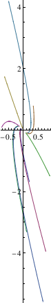
We want to show this instability by constructing a finite number of solutions, which we can obtain from the general solution by specifying the initial conditions. We choose, for instance, 8 points, as initial conditions that the solution plot will go through:

initlist2 = {{5, 1}, {5, 2}, {-5, 1}, {-5, 2}, {-5, -1}, {-5, -2}, {5, -1}, {5, -2}};
For constant coefficient differential equations, solutions exist for all t from minus infinity to infinity. However, when we use initial conditions at our specified 8 points, we encounter the problem that our solutions diverge to infinity. Obviously, our plotting window cannot be expanded infinitely to show all solutions. As t goes to negative infinity, our solution approaches the origin, which means we need to incorporate negative time in our plotting. We use t = -6 for simplicity. We take the coordinates in the above list to be initial positions at t = 0, and then we integrate over a time interval {-6, 0}. NDSolve will begin the integration at t = 0, and then go back in time to t = -6, thus tracing the 
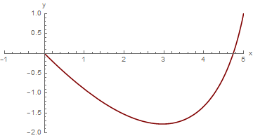
solution back in time. Let's try this for one solution before generating all 8. First we define the equation as a function of the initial values.
equation2[x0_, y0_] := {x'[t] == x[t] - y[t], y'[t] == 3 x[t] + 5 y[t], x[0] == x0, y[0] == y0}
{xtest, ytest} = {x[t], y[t]} /. Flatten[NDSolve[equation2[5, 1], {x[t], y[t]}, {t, -6, 0}]]
testgraph2 = ParametricPlot[{xtest, ytest}, {t, -6, 0}, PlotRange -> {{-1, 5}, {-2, 1}},
AxesLabel -> {"x", "y"}, AspectRatio -> Automatic, PlotStyle -> RGBColor[1/2, 0, 0]]
We see that this solution starts very near the origin at t = -6, and has progressed to the point {5,1} when t has increased to 0. 
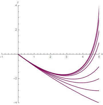
Now we construct graphs of all of the other solutions with the given initial conditions in initlist2 -- 8 solutions in all based on our 8 initial conditions. We first define a routine that calculates and then graphs a solution for a given set of initial conditions.
graph2[x0_, y0_] :=
Module[{xans,
yans}, {xans, yans} = {x[t], y[t]} /.
Flatten[NDSolve[equation2[x0, y0], {x[t], y[t]}, {t, -6, 0}]]; ParametricPlot[{xans, yans}, {t, -6, 0},
PlotRange -> {{-1, 5}, {-2, 1}}, AxesLabel -> {"x", "y"}, AspectRatio -> Automatic, PlotStyle -> RGBColor[1/2, 0, 1/3]]]
Upon typing graph2[5, 1], we get exactly the same figure using different code. Our routine works, but when we apply it to get our 8 solutions, we are going to get individual graphs of each. Instead, we want to create a composite graph of all 8 solutions. We can do this by telling our basic graph routine NOT to display the graph it creates. This is accomplished using the option DisplayFunction -> Identity.
graph2z[x0_, y0_] :=
Module[{xans, yans}, {xans, yans} = {x[t], y[t]} /.
Flatten[NDSolve[equation2[x0, y0], {x[t], y[t]}, {t, -6, 0}]]; ParametricPlot[{xans, yans}, {t, -6, 0}, PlotRange -> {{-1, 5}, {-2, 1}}, AxesLabel -> {"x", "y"},
AspectRatio -> Automatic, DisplayFunction -> Identity, PlotStyle -> RGBColor[1/2, 1/2, 1/2]]]
We try it again.
testgraph2z = graph2z[5, 1]
Our modification has been successful, so we can now use the Show command with the option DisplayFunction->$DisplayFunction, which tells Mathematica to show the graph.
Show[testgraph2z, DisplayFunction -> $DisplayFunction]
Now we are going to use a Do loop to create all 8 graphs, without showing them individually. At the end we will show them all together, and after that, we will combine them with the direction field. We collect the graphs in a list named graphlist2.
Module[{i, x0temp, y0temp, pair, newgraph}, graphlist2 = {};
Do[pair = initlist2[[i]];
x0temp = Part[pair, 1]; y0temp = Part[pair, 2];
newgraph = graph2[x0temp, y0temp];
graphlist2 = Append[graphlist2, newgraph], {i, 1, 8}]]
Now we plot them
Show[testgraph2z, DisplayFunction -> $DisplayFunction]

We now consider the system \( \dot{\bf y} (t) = {\bf A}\, {\bf y} , \) where square matrix A has a complex eigenvalue λ = α + jβ with β ≠ 0. As usual, we assume that A has real entries, so the characteristic polynomial det(λIA) of matrix A has real coefficients. This implies that its complex conjugate α − jβ is also N eigenvalue of A.

An eigenvector x of A associated with λ = α + jβ has complex entries,

\[ {\bf x} = {\bf u} + {\bf j}\,{\bf v} , \]
where u and v have real entries; so u and v are the real and imaginary parts of x. Since A x = λx, we have
\[ {\bf A}\,{\bf x} = {\bf A} \left( {\bf u} + {\bf j}\,{\bf v} \right) = \left( \alpha + {\bf j}\,\beta \right) \left( {\bf u} + {\bf j}\,{\bf v} \right) . \]
Taking complex conjugate here and recalling that A has real entries yields
\[ {\bf A}\,\overline{\bf x} = {\bf A} \left( {\bf u} - {\bf j}\,{\bf v} \right) = \left( \alpha - {\bf j}\,\beta \right) \left( {\bf u} - {\bf j}\,{\bf v} \right) , \]
which shows that ujv is an eigenvector associated with \( \overline{\lambda} = \alpha - {\bf j}\beta . \)
Theorem 1: Let A be an n × n matrix with real entries. Let λ = α + jβ (β ≠ 0) be a complex eigenvalue of A and let x = u + j v be an associated eigenvector, where u and v have real components. Then u and v are both nonzero and
\[ {\bf y}_1 = e^{\alpha\,t} \left( {\bf u} \,\cos \beta t - {\bf v}\,\sin \beta t \right) \qquad \mbox{and} \qquad {\bf y}_2 = e^{\alpha\,t} \left( {\bf u} , \,\sin \beta t + {\bf v}\,\cos \beta t \right) \]
which are real and imaginary parts of
\[ e^{\alpha\,t} \left( \cos \beta t + {\bf j}\,\sin \beta t \right) \left( {\bf u} + {\bf j}\,{\bf v}\right) \]
are linearly independent solutions of \( \dot{\bf y} (t) = {\bf A}\, {\bf y} . \)
A function of the form
\[ {\bf y}(t) = f_1 (t)\,{\bf u} + f_2 (t)\,{\bf v} \]
is a solution of the system of equations \( \dot{\bf y} (t) = {\bf A}\, {\bf y} \) if and only if
\[ \dot{f}_1 (t)\,{\bf u} + \dot{f}_2 (t)\,{\bf v} = f_1 (t)\,{\bf A}\,{\bf u} + f_2 (t)\,{\bf A}\,{\bf v} . \]
Carring out the multiplication and collecting the real and imaginary [arts, we get
\[ {\bf A} \left( {\bf u} + {\bf j\,v} \right) = \left( \alpha {\bf u} - \beta {\bf v} \right) + {\bf j} \left( \alpha {\bf v} + \beta {\bf u} \right) . \]
Equating real and imaginary parts on the sides of this equation yields
\[ \begin{cplit} {\bf A}\,{\bf u} &= \alpha {\bf u} - \beta {\bf v} , \\ {\bf A}\,{\bf v} &= \alpha {\bf v} + \beta {\bf u} . \end{split} \]
Example 5: Consider another system of differential equations whose coefficient matrix has complex conjugate eigenvalues: \( {\bf A} = \begin{bmatrix} \phantom{-}1&1 \\ -1&1 \end{bmatrix} . \)
A = {{1, 1}, {-1, 1}}
Out[10]= {{1, 1}, {-1, 1}}
Eigenvalues[A]
Out[11]= {1 + I, 1 - I}

We solve this system and plot some solutions in a similar way as in the previous example

X[t_] = {x[t], y[t]}
Out[12]= {x[t], y[t]}
system = MapThread[#1 == #2 &, {X'[t], A.X[t]}]
Out[13]= {Derivative[1][x][t] == x[t] + y[t],
Derivative[1][y][t] == -x[t] + y[t]}
sol = DSolve[system, {x, y}, t]
Out[14]= {{x -> Function[{t}, E^t C[1] Cos[t] + E^t C[2] Sin[t]],
y -> Function[{t}, E^t C[2] Cos[t] - E^t C[1] Sin[t]]}}
      Then we plot some solution curves
particular =
Partition[
Flatten[Table[{x[t], y[t]} /. sol /. {C[1] -> 1/i,
C[2] -> 1/j}, {i, -20, 20, 7}, {j, -20, 20, 7}]], 2];
ParametricPlot[Evaluate[particular], {t, -33, 33}, PlotRange -> All,
PlotPoints -> 70, Method -> {Compiled -> False}]
       Some solution curves.            Mathematica code

The spiraling behavior is typical for systems with complex eigenvalues.
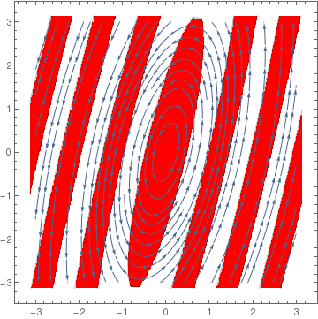
Example 6: Consider a linear system of ordinary differential equations
\[ \dot{x} = x-y , \qquad \dot{y} = 5\,x -y. \]
The corresponding matrix \( \begin{bmatrix} 1 & -2 \\ 5 & -1 \end{bmatrix} \) has two pure imaginary eigenvalues \( \lambda = \pm 2{\bf j} , \) where j is the unit vector in the positive vertical direction on the complex plane.

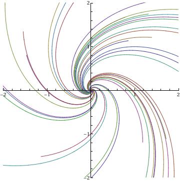
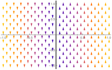
Using the standard Mathematica command StreamPlot, we visualize a phase portrait for the given system

StreamPlot[{x - y, 5*x - y}, {x, -3, 3}, {y, -3, 3}, Mesh -> 7, MeshShading -> {Red, None}]
As we see, trajectories circle around the origin in a counterclockwise direction. If we use the negative of matrix A, trajectories will circle the origin in clockwise direction.
StreamPlot[{-x + y, -5*x + y}, {x, -3, 3}, {y, -3, 3}, FrameLabel -> {x, y}]
   ■


Singular Matrices


If matrix A is invertible, then the only critical point of the homogeneous linear differential equation dy/dt = Ay is the origin. However, when matrix A is singular, then Eq.\eqref{EqConstant.1} has infinite many critical non-isolated points because the algebraic equation Ay = 0 defines non-trivial null-space of matrix A. We illustrate this situation with the following examples.
Example 7: We consider the singular matrices
\[ {\bf A} = \begin{bmatrix} 1&-3 \\ 2&-6 \end{bmatrix} \qquad {\bf B} = \begin{bmatrix} 1&2 \\ 2&4 \end{bmatrix} , \qquad \mbox{and} \qquad {\bf C} = \begin{bmatrix} -2&0 \\ \phantom{-}0&0 \end{bmatrix} \]
that are used to solve the system of differential equations \eqref{EqConstant.1}.

Example 7A: Matrix A has two eigenvalues λ = 0 and λ = −5.

A = {{1, -3}, {2, -6}}
Eigenvalues[A]
{-5, 0}
Next, we determine its eigenvectors with Mathematica:
A = {{1, -3}, {2, -6}}
Eigenvectors[A]
{{1, 2}, {3, 1}}
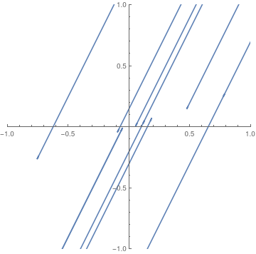
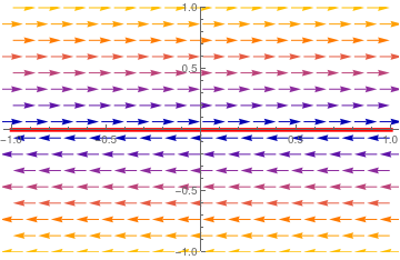
So we know that the eigenspace corresponding to the eigenvalue λ = 0 is spanned on the vector [3, 1]T. Every vector from this eigenspace is a critical point for the system of equations
\[ \frac{{\text d}{\bf y}}{{\text d}t} = {\bf A}\,{\bf y} \qquad \mbox{or} \qquad \frac{{\text d}}{{\text d}t} \begin{bmatrix} y_1 (t) \\ y_2 (t) \end{bmatrix} = \begin{bmatrix} y_1 (t) - 3\, y_2 (t) \\ 2\,y_1 (t) - 6\,y_2 (t) \end{bmatrix} . \tag{7.1} \]
The general solution of Eq.(7.1) is
A = {{1, -3}, {2, -6}}
MatrixExp[A*t]
{{6/5 - E^(-5 t)/5, -(3/5) + (3 E^(-5 t))/5}, {2/5 - (2 E^(-5 t))/ 5, -(1/5) + (6 E^(-5 t))/5}}
\[ {\bf y} (t) = e^{{\bf A}t} {\bf c} , \qquad \mbox{where} \qquad e^{{\bf A}t} = \frac{1}{5} \begin{bmatrix} 6 - e^{-5t} & 3\, e^{-5t} - 3 \\ 2 - 2\, e^{-5t} & 6\, e^{-5t} -1 \end{bmatrix} , \]
and c is a vector of two arbitrary real constants. First, we plot some solutions. First, we make a modul for plotting solutions of a two-dimensional system of equations \eqref{EqConstant.1}.
TrajectoryPlot[system_, initialPts_, {time_, tMin_, tMax_}, {xVar_, xMin_, xMax_}, {yVar_, yMin_, yMax_}] := Module[{}, Off[NDSolve::ndsz]; Off[InterpolatingFunction::dmval];
getSolution[k_] := First[NDSolve[ Join[system, {x[0] == initialPts[[k, 1]], y[0] == initialPts[[k, 2]]}], {x, y}, {t, tMin, tMax}]]; getEstDomain[funct_] := {t, Flatten[funct[[1]]][[1]] + 0.2, Flatten[funct[[1]]][[2]] - 0.2};
Block[{$DisplayFunction = Identity}, solutionList = Table[ParametricPlot[Evaluate[{x[t], y[t]} /. getSolution[k]], Evaluate[getEstDomain[x /. getSolution[k]]], PlotRange -> {{xMin, xMax}, {yMin, yMax}}, AspectRatio -> Automatic, PlotPoints -> 100], {k, 1, Length[initialPts]}];]; On[NDSolve::ndsz];
Show[solutionList]]
      We define a set of points on the plane that will be used as the initial points for solutions.
points = {{0.7, 0.1}, {0.6, 0.4}, {0.8, 0.3}, {0.2, 0.2}, {0.1, 0.1}, {-.6, .05}, {-.05, .05}, {-0.1, -0.5}, {-0.2, -0.6}, {-0.3, \ -0.5}, {-0.3, -0.5}}
Finally, we plot solutions.
f[x_, y_] = x - 3*y; g[x_, y_] = 2*x - 6*y;
solCurves = TrajectoryPlot[{x'[t] == f[x[t], y[t]], y'[t] == g[x[t], y[t]]}, points, {t, -100, 100}, {x, -1, 1}, {y, -1, 1}]
       Some solutions of Eq.(7.1).            Mathematica code

Next, we plot the direction field for system (7.1) along with the separatrix (in red), which is the null-space of matrix A.
      We plot the direction field corresponding to matrix A.
vp = VectorPlot[{x - 3*y, 2*x - 6*y}, {x, -1, 1}, {y, -1, 1}]
null = Plot[x/3, {x, -1, 1}, PlotStyle -> {Thickness[0.01], Red}]
Show[null, vp]
       Direction field with the separatrix (in red).            Mathematica code


Example 7B: Two linearly independent solutions to the system of differential equations

\[ \dot{x} = x + 2\,y , \qquad \dot{y} = 2\,x + 4\,y \]
are
y1[t_] = Exp[lambda1*t]*v1
{E^(5 t), 2 E^(5 t)}
y2[t_] = Exp[lambda2*t]*v2
{-2, 1}
So its fundamental matrix becomes
\[ e^{{\bf B}\,t} = \begin{bmatrix} e^{5t} & -2 \\ 2\,e^{5t} & 1 \end{bmatrix} , \qquad \blacksquare \]


Example 7C: Matrix C is diagonalizable because it is a diagonal matrix itself. Its eigenvalues

CC = {{-2, 0}, {0, 0}}
Eigenvalues[CC]
{-2, 0}
are λ = −2 and λ = 0, to which correspond eigenvectors
CC = {{-2, 0}, {0, 0}}
Eigenvectors[CC]
{{1, 0}, {0, 1}}
      We plot the direction field corresponding to matrix C along with the separatrix (in orange) that consists of scritical points.
vp = VectorPlot[{-2*x, 0}, {x, -1, 1}, {y, -1, 1}]
line = Plot[None, {x, -1, 1}, Axes -> False, Epilog -> {Thickness[0.01], Orange, Line[{{0, -1}, {0, 1}}]}]
Show[line, vp]
       Direction field with the separatrix (in orange).            Mathematica code

The expnential matrix is diagonal
\[ e^{{\bf C}t} = \begin{bmatrix} e^{-2t} & 0 \\ 0 & 1 \end{bmatrix} . \]
CC = {{-2, 0}, {0, 0}}
MatrixExp[CC*t]
{{E^(-2 t), 0}, {0, 1}}
   ■
Example 8: We consider three nilpotent matrices (a square matrix is called nilpotent if its some power is the zero matrix; in two dimensional case, this means that the matrix must have both, trace and determinant, to be zeroes)
\[ {\bf A} = \begin{bmatrix} 0&2 \\ 0&0 \end{bmatrix} , \qquad {\bf B} = \begin{bmatrix} 0&0 \\ 2&0 \end{bmatrix} , \qquad \mbox{and} \qquad {\bf T} = \begin{bmatrix} 2&-4 \\ 1&-2 \end{bmatrix} . \]
First, we check that all matrices are nilpotent.
A = {{0,2},{0,0}}
A.A
{{0, 0}, {0, 0}}
B = {{0,0},{2,0}}
B.B
{{0, 0}, {0, 0}}
T = {{2,-4},{1,-2}}
T.T
{{0, 0}, {0, 0}}
Nilpotent matrices are not diagonalizable, so we check with Mathematica their eigenvectors.
Eigenvalues[A]
{0, 0}
Eigenvectors[A]
{{1, 0}, {0, 0}}
Eigenvalues[B]
{0, 0}
Eigenvectors[B]
{{0, 1}, {0, 0}}
Eigenvalues[T]
{0, 0}
Eigenvectors[T]
{{2, 1}, {0, 0}}


Let us consider matrix A.
      We plot the direction field along with the separatrix (in red).
vp = VectorPlot[{2*y, 0}, {x, -1, 1}, {y, -1, 1}]
line = Plot[y[x] = 0, {x, -1, 1}, PlotRange -> {-1, 1}, PlotStyle -> {Thickness[0.01], Red}]
Show[line, vp]
       Direction field and separatrix (in red).            Mathematica code

The exponential matrix that corresponds to A is
\[ e^{{\bf A}t} = \begin{bmatrix} 1 & 2t \\ 0 & 1 \end{bmatrix} . \]
A = {{0,2},{0,0}}
MatrixExp[A*t]
{{1, 2 t}, {0, 1}}


The nilpotent matrix B has only one linearly independent eigenvector that is spanned on [0, 1]T.
      We plot the direction field corresponding to matrix B.
line = Plot[None, {t, -1, 1}, GridLines -> {{0}}, GridLinesStyle -> { Thickness[0.01], Red}]
vp = VectorPlot[{0, 2*x}, {x, -1, 1}, {y, -1, 1}]
Show[line, vp]
       Direction field with the separatrix (in red).            Mathematica code

The exponential matrix that corresponds to B is
\[ e^{{\bf B}t} = \begin{bmatrix} 1 & 0 \\ 2\,t & 1 \end{bmatrix} . \]
MatrixExp[B*t]
{{1, 0}, {2 t, 1}}


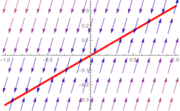
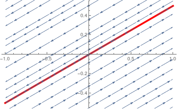
We know that matrix T is a defective matrix with only one linearly independent eigenvector [2, 1]T corresponding to double eigenvalue λ = 0. Next, we plot the direction field for system (7.1) along with the separatrix (in red), which is the null-space of matrix T.
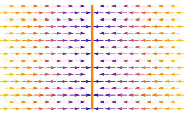
      We plot the direction field corresponding to matrix C.
T = {{2, -4}, {1, -2}}
sp = StreamPlot[{2*x - 4*y, x - 2*y}, {x, -1, 1}, {y, -1, 1}]
null = Plot[x/2, {x, -1, 1}, PlotStyle -> {Thickness[0.01], Red}]
Show[null, sp]
       Direction field with the separatrix (in red).            Mathematica code

Its exponential matrix is
\[ e^{{\bf T}t} = \begin{bmatrix} 1 + 2t & -4t \\ t & 1-2t \end{bmatrix} . \]
MatrixExp[T*t]
{{1 + 2 t, -4 t}, {t, 1 - 2 t}}
   ■
Example 9:    ■


Return to Mathematica page
Return to the main page (APMA0340)
Return to the Part 1 Matrix Algebra
Return to the Part 2 Linear Systems of Ordinary Differential Equations
Return to the Part 3 Non-linear Systems of Ordinary Differential Equations
Return to the Part 4 Numerical Methods
Return to the Part 5 Fourier Series
Return to the Part 6 Partial Differential Equations
Return to the Part 7 Special Functions