ch7 MATHEMATICA tutorial, Part 2: Converting to a system

Return to computing page for the first course APMA0330
Return to computing page for the second course APMA0340
Return to Mathematica tutorial for the first course APMA0330
Return to Mathematica tutorial for the second course APMA0340
Return to the main page for the first course APMA0330
Return to the main page for the second course APMA0340
Introduction to Linear Algebra with Mathematica

Preface


This section presents the concept of converting a single ordinary differential equation (linear or nonlinear) into an equivalent system of first order differential equations. More precisely, if a single differential equation in normal form is of order n, then it is possible to transfer it to an equivalent system containing n (or more) differential equations of first order. Although this conversion is not unique, it is always the case that the single equation and the system of differential equations have the same set of solutions. Moreover, upon introducing additional auxiliary dependent variables, it is possible to simplify the problem and/or obtain useful information about solutions.

The reverse procedure of converting a system of linear ODEs into a single equation is discussed in section viii of Part 2. Not every system of n linear first order differential equations can be transfered to a single n-th order differential equation.

Converting to a system


Given a single ordinary differential equation, one method of finding numerical solutions entails transferring it into an equivalent system of differential equations of the first order. When a single differential equation has an isolated highest derivative, it is always possible to transfer the differential equation into an equivalent system of differential equations of the first order. This can be achieved by denoting sequential derivatives of the unknown variable with a new dependent variable with the exception of the last derivative, which is used to incorporate the given single differential equation. Other options are also possible for such a conversion, which will be clear from the examples.

The word "equivalent" indicates that both a single differential equation and the corresponding system of equations have the same set of solutions (so no solution is lost or added). The opposite is not always true, and some systems of n ordinary differential equations cannot be reduced to an equivalent single n-th order differential equation. The general solution of the single n-th order differential equation depends on n arbitrary constants and it belongs to the space of functions having n continuous derivatives, which is usually denoted by Cn. A system of n differential equations has the same properties and its general solution also depends on n arbitrary constants. Therefore, a single n-th order ODE can be equivalent to the system of (n+1) first order ODEs only when the latter does not require extra differentiation of the unknown function. However, a single n-th order ODE cannot be equivalent to the (n−1) system of first order ODEs because the latter contains (n−1) arbitrary constants and requires utilization of Cn-1. A key illustration highlighting this is the pendulum equation, presented in Example 5, which does not use the derivative operator, and where a single second order equation is transformed into four first order equations representing an equivalent system. On the other hand, the derivative operator is used in Example 1, showing that the resulting system of equations is not equivalent to the original equation. Therefore, the key takeaway is to avoid using the derivative operator because it is an unbounded operation.

There are a couple of reasons why it is convenient to transfer a single differential equation of an order higher than one to a system of differential equations of first order. First of all, it is simpler to analyze theoretically the first order vector differential equation than deal with a higher order differential equation because the latter can be naturally included into a broader topic: systems of differential equations. Second, it is easier to use and implement a universal numerical algorithm for a first order derivative operator instead of utilizing special numerical procedures for higher order derivatives. It is more accurate to monitor errors of numerical calculations for a system of first order differential equations than for a single equation. Also, there are many situations in which we not only want to know the solution to an ODE (acronym for Ordinary Differential Equations), but also the derivative or acceleration of the solution. This information can be naturally extracted from the solution to the system of first order differential equations (with no extra work).

When treating the independent variable as a time, it is common to use Newton's notation \( \dot{y} \) for the derivative instead of Lagrange notation y' or Leibniz's notation \( \displaystyle {\text d}y/{\text d}t . \) Sometimes, we also utilize Euler's notation for the derivative operator: \( \displaystyle \texttt{D} = {\text d}/{\text d}t . \)

Example 1: Let us start with a simple case of constant coefficient linear differential equation when all manipulations become transparent. So we consider the following initial value problem for a linear second order differential equation
\begin{equation*} %\label{EqConv.1} x''(t) + 2x'(t) - 3x(t) = 0, \qquad x(0) =3, \quad x' (0) =-1. \tag{1.1} \end{equation*}
This is a homogeneous, linear, second-order ODE with constant coefficients. As a brief refresher from the previous course, recall that its solution can be computed by finding the roots of the corresponding characteristic equation:
\[ \lambda^2 + 2\,\lambda - 3 = 0. \tag{1.2} \]
There are two distinct, real roots to the quadratic (characteristic) equation: λ1 = 1 and λ2 = -3, and the general solution is a linear combination of two exponent functions:
\[ x(t) = c_{1}e^{\lambda_{1}t} + c_{2}e^{\lambda_{2}t} = c_{1}e^{t} + c_{2}e^{-3t} , \]
where c1 and c2 are arbitrary constants. To satisfy the initial conditions, we have to choose these constants so that x(0) = c1 + c2 = 3 and x'(0) = c1 -3 c2 = -1. This yields c1 = 2 and c2 = 1; and the solution becomes
\begin{equation*} %\label{EqConv.2} x(t) = 2\, e^t + e^{-3t} \qquad \Longrightarrow \qquad x'(t) = 2\, e^t -3\, e^{-3t} . \tag{1.3} \end{equation*}
DSolve[{x''[t] + 2*x'[t] - 3*x[t] == 0, x[0] == 3, x'[0] == -1}, x[t], t]
Now we convert the given problem to a vector equation by letting x1 = x and its first derivative we denote by x2. Note that second derivative is known from the given equation \( x'' = 3\,x(t) - 2\, x' (t) = 3\, x_1 - 2\, x_2 . \) This leads to the system of first order differential equations
\[ \begin{split} x'_1 &= x_2 = x', \\ x'_2 &= x'' = -2\, x_2 + 3\,x_1 . \end{split} \]
Upon introducing a column vector x = [ x1, x2]T (here "T" stands for transposition; see first chapter of this tutorial), we can rewrite the system of ODEs in a more appropriate vector form:
\begin{equation*} %\label{EqConv.3} \frac{\text d}{{\text d}t} \begin{bmatrix} x_1 (t) \\ x_2 (t) \end{bmatrix} = \begin{bmatrix} 0& \phantom{-}1 \\ 3 & -2 \end{bmatrix} \begin{bmatrix} x_1 (t) \\ x_2 (t) \end{bmatrix} , \qquad \begin{bmatrix} x_1 (0) \\ x_2 (0) \end{bmatrix} = \begin{bmatrix} \phantom{-}3 \\ -1 \end{bmatrix} . \tag{1.4} \end{equation*}
DSolve[{x1'[t] == x2[t], x2'[t] == -2*x2[t] + 3*x1[t], x1[0] == 3, x2[0] == -1}, {x1[t], x2[t]}, t]
{{x1[t] -> E^(-3 t) (1 + 2 E^(4 t)), x2[t] -> E^(-3 t) (-3 + 2 E^(4 t))}}
With matrix notation,
\[ {\bf x} (t) = \begin{bmatrix} x_1 (t) \\ x_2 (t) \end{bmatrix} , \qquad {\bf A} = \begin{bmatrix} 0& \phantom{-}1 \\ 3 & -2 \end{bmatrix} , \qquad {\bf x}_0 = \begin{bmatrix} \phantom{-}3 \\ -1 \end{bmatrix} , \]
we rewrite the system of ODEs and corresponding initial conditions in compact form:
\[ \frac{\text d}{{\text d}t}\,{\bf x}(t) = {\bf A}\,{\bf x}(t) , \qquad {\bf x}(0) = {\bf x}_0 . \]
In order to find the solution to this vector differential equation, we first need to find the eigenvalues of the corresponding matrix (which is called the companion matrix):
\[ \det \left( \lambda {\bf I} - {\bf A} \right) =0 \qquad \Longleftrightarrow \qquad \det \left( \lambda \begin{bmatrix} 1&0 \\ 0&1 \end{bmatrix} - \begin{bmatrix} 0&\phantom{-}1 \\ 3&-2 \end{bmatrix} \right) = \det \begin{bmatrix} \lambda & -1 \\ -3& \lambda +2 \end{bmatrix} = \lambda^2 + 2\,\lambda - 3 =0 , \]
where I is the identity matrix. From observation, the eigenvalues of matrix A are the same as the roots of the characteristic equation λ² + 2 λ −3 = 0 for the given second order differential equation.

Sometimes, we need to monitor the residual of numerical calculations by introducing an additional auxiliary variable y3 = x'', the second derivative of the unknown solution x(t), and keep other variables: y1 = x and y2 = x'. Then its derivative, according to the given differential equation, will be:

\[ y'_3 = x''' = \frac{\text d}{{\text d}t} \left( x'' \right) = \frac{\text d}{{\text d}t} \left( -2\,y_2 + 3\, y_1 \right) = -2\,y'_2 + 3\, y'_1 = -2 \left( -2\, y_2 + 3\, y_1 \right) + 3\, y_2 = 7\, y_2 -6\, y_1 . \]
This allows us to compose the system of three equations. There are two options to achieve it. First, we recall that the derivative of y2 is our new dependent variable y3. So we get
\begin{equation*} %\begin{split} \begin{cases} y'_1 &= y_2 = x' , \\ y'_2 &= y_3 = x'' , \\ y'_3 &= -2\, y_3 +3 \, y_2 = x''' ; \end{cases} %\end{split} \qquad\quad %\begin{split} \begin{cases} y_1 (0) &= 3 \\ y_2 (0) &= -1 \\ y_3 (0) &= 11 . \end{cases} %\end{split} \tag{1.5} \end{equation*}
Therefore, we obtain a vector differential equation \( \dot{\bf y} = {\bf C}\,{\bf y}(t) \) that is equivalent (we hope?) to the the original IVP (1.1)
\[ \frac{\text d}{{\text d}t} \begin{bmatrix} y_1 (t) \\ y_2 (t) \\ y_3 (t) \end{bmatrix} = \begin{bmatrix} 0&1&\phantom{-}0 \\ 0&0&\phantom{-}1 \\ 0&3&-2 \end{bmatrix} \begin{bmatrix} y_1 (t) \\ y_2 (t) \\ y_3 (t) \end{bmatrix} , \qquad \begin{bmatrix} y_1 (0) \\ y_2 (0) \\ y_3 (0) \end{bmatrix} =\begin{bmatrix} \phantom{1}3 \\ -1 \\ 11 \end{bmatrix} , \qquad\mbox{with}\quad {\bf C} = \begin{bmatrix} 0&1&\phantom{-}0 \\ 0&0&\phantom{-}1 \\ 0&3&-2 \end{bmatrix} . \]
The initial condition for this function also follows from the given differential equation (1.1):
\[ y_3 = x'' = 3\, x(t) - 2\, x' (t) \qquad \Longrightarrow \qquad y_3 (0) = 3\,x(0) -2\, x' (0) = 3\cdot 3 -2 \cdot (-1) = 11 . \]
Note that the derivative of y3 is expressed through the original function x(t) as \( y'_3 = 7\, y_2 -6\, y_1 . \) So another option is to rewrite the given system of ODEs as
\begin{equation*} %\label{EqConv.4} %\begin{split} \begin{cases} y'_1 &= y_2 = x' , \\ y'_2 &= y_3 = x'' , \\ y'_3 &= -6\, y_1 +7\, y_2 = x''' ; \end{cases} %\end{split} \qquad\quad %\begin{split} \begin{cases} y_1 (0) &= 3 \\ y_2 (0) &= -1 \\ y_3 (0) &= 11 . \end{cases} %\end{split} \tag{1.6} \end{equation*}
In vector form, it becomes:
\[ \frac{\text d}{{\text d}t} \begin{bmatrix} y_1 (t) \\ y_2 (t) \\ y_3 (t) \end{bmatrix} = \begin{bmatrix} \phantom{-}0&1&0 \\ \phantom{-}0&0&1 \\ -6&7&0 \end{bmatrix} \begin{bmatrix} y_1 (t) \\ y_2 (t) \\ y_3 (t) \end{bmatrix} , \qquad \begin{bmatrix} y_1 (0) \\ y_2 (0) \\ y_3 (0) \end{bmatrix} =\begin{bmatrix} \phantom{1}3 \\ -1 \\ 11 \end{bmatrix} , \qquad\mbox{with}\quad {\bf B} = \begin{bmatrix} \phantom{-}0&1&0 \\ \phantom{-}0&0&1 \\ -6&7&0 \end{bmatrix} . \]
DSolve[{y1'[t] == y2[t], y2'[t] == -2*y2[t] + 3*y1[t], y3'[t] == 7*y2[t] - 6*y1[t], y1[0] == 3, y2[0] == -1, y3[0] == 11}, {y1[t], y2[t], y3[t]}, t]
{{y1[t] -> E^(-3 t) (1 + 2 E^(4 t)), y2[t] -> E^(-3 t) (-3 + 2 E^(4 t)), y3[t] -> E^(-3 t) (9 + 2 E^(4 t))}}
Despite that the first two components (y1 and y2) of the solution to the initial value problem (1.6) are the same as (1.3),
\[ \begin{bmatrix} y_1 (t) \\ y_2 (t) \\ y_3 (t) \end{bmatrix} = \begin{bmatrix} e^{-3t} + 2\,e^{t} \\ -3\,e^{-3t} + 2\,e^{t} \\ 9\,e^{-3t} + 2\,e^{t} \end{bmatrix} , \]
the system of diferential equations (1.6) is not equivalent to (1.1) because the corresponding matrix B has three eigenvalues {−3, 2, 1}. Recall that matrix A has two eigenvalues {−3, 1}. It becomes clear when we rewrite the system of three equations with matrix B in the following form with Euler's notation \( \texttt{D} = {\text d}/{\text d}t \) for derivative operator:

\[ \begin{split} \texttt{D} y_1 &= y_2 , \\ \texttt{D} y_2 &= y_3 , \\ \texttt{D} y_3 &= -6\,y_1 + 7\,y_2 . \end{split} \]
The system above contains three unbounded derivative operators, but the original differential equation (1.1) is of order two. So its general solution is
\[ y_1 (t) = x(t) = C_1 e^t + C_2 e^{-3t} + C_3 e^{2t} , \]
with some arbitrary constants C1, C2, and C3. Upon using the appropriate initial conditions we eliminated unwanted additional constant C3 from its general solution. So we obtain the same solution from the system of three equations as the original IVP, at least from theoretical point of view. However, matrix B has a dominant eigenvalue λ = 2>1 and the corresponding numerical algorithm should avoid it.

Then the difference of y3 and \( 3\, x(t) - 2\,x' (t) = 3\,y_1 - 2\, y_2 \) gives the residual (error) of calculations.

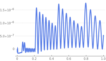
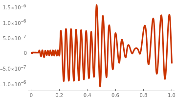
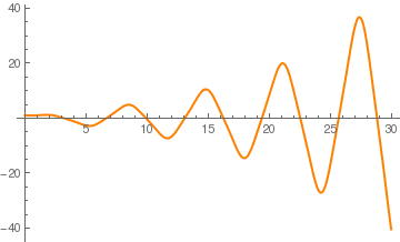
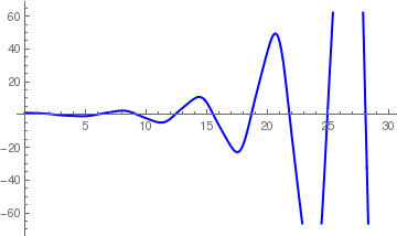
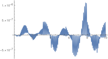
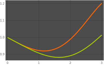
We use the standard Mathematica command NDSolve to solve numerically the system of three equations (1.6) and plot the residual of calculations for the equation. Blue curve gives the error with the true second derivative, and the red curve gives the residual based on numerical calculation.

sol3 = NDSolve[{y1'[t] == y2[t], y2'[t] == y3[t], y3'[t] == -6*y1[t] + 7*y2[t], y1[0] == 3, y2[0] == -1, y3[0] == 11}, {y1, y2, y3}, {t, 0, 3}];
sol2 = NDSolve[{x1'[t] == x2[t], x2'[t] == 3*x1[t] - 2*x2[t], x1[0] == 3, x2[0] == -1}, {x1, x2}, {t, 0, 3}];
a1 = Plot[ Evaluate[y3[t] /. sol3] + Evaluate[(2*x2[t] - 3*x1[t]) /. sol2], {t, 0, 1}, PlotTheme -> "Web"]
a2 = Plot[9 E^(-3 t) + 2 E^t - Evaluate[(y3[t]) /. sol3], {t, 0, 1}, PlotTheme -> "Business"]
     
       Figure 1. Residuals of the second derivative: the error between the second derivative y3(t) and the true value in blue.              Figure 2. The residual of the second derivative y3(t) = d²x/dt² and the numerical solution 3x2(t) - 2x1(t).

Note that introducing the system of three equations with artificial differentiation does not provide an equivalent system for the given equation because the derivative operator is unbounded.

The transformation to a system of first order ODEs is straight forward, but it is not unique. Let us try another set of new dependent variables:

\[ z_1 = x, \quad z_2 = \dot{x} - x \qquad\Longrightarrow \qquad \dot{z}_2 = \ddot{x} - \dot{x} = -3 \left( \dot{x} - x \right) . \]
This leads to the system of first order differential equations:
\[ \begin{split} \dot{z}_1 &= z_1 + z_2 \qquad \Longleftrightarrow \qquad \dot{x} = \dot{x} , \\ \dot{z}_2 &= -3\, z_2 . \end{split} \]
We can also rewrite the above system in vector form
\[ \frac{\text d}{{\text d}t} \begin{bmatrix} z_1 (t) \\ z_2 (t) \end{bmatrix} = \begin{bmatrix} 1& \phantom{-}1 \\ 0 & -3 \end{bmatrix} \begin{bmatrix} z_1 (t) \\ z_2 (t) \end{bmatrix} , \qquad \begin{bmatrix} z_1 (0) \\ z_2 (0) \end{bmatrix} = \begin{bmatrix} \phantom{-}3 \\ -4 \end{bmatrix} , \]
because \( z_2 (0) = \dot{x}(0) - x(0) = -1 -3 =-4 . \) The characteristic polynomial for the corresponding matrix is
\[ \det \left( \lambda \begin{bmatrix} 1&0 \\ 0&1 \end{bmatrix} - \begin{bmatrix} 1&\phantom{-}1 \\ 0&-3 \end{bmatrix} \right) = \det \begin{bmatrix} \lambda -1& -1 \\ 0& \lambda +3 \end{bmatrix} = \lambda^2 + 2\,\lambda - 3 =0 . \]
Example 1A: We consider a similar differential equation, but now it is a nonhomogeneous equation:
\begin{equation*} %\label{EqConv.1a} x''(t) + 2x'(t) - 3x(t) = 10\,\sin t, \qquad x(0) =3, \quad x' (0) =-1. \tag{1A.1} \end{equation*}
This is an inhomogeneous, linear, second-order ODE with constant coefficients. We find its particlular solution using method of undetermined coefficients:
\[ x_p (t) = A\,\cos t + B\,\sin t . \]
Numerical values of coefficients A and B are determined upon substitution xp into the given differential equation:
\[ -4 \left( A\,\cos t + B\,\sin t \right) + 2 \left( -A\,\sin t + B\,\cos t \right) = 10\,\sin t . \]
Equating coefficients of sine and cosine functions (that are linearly independent), we obtain the following system of algebraic equations:
\[ -4A + 2B =0, \qquad -4B -2A =10 . \]
Solve[{-4*A + 2*B == 0, -4*B - 2*A == 10}, {A, B}]
{{A -> -1, B -> -2}}
Using Mathematica, we get the general solution to be
\[ x(t) = c_{1}e^{t} + c_{2}e^{-3t} - \cos t -2\,\sin t, \]
where c1 and c2 are arbitrary constants. Substitution of the general solution into the initial conditions yields
\[ x(0) = c_{1} + c_{2} -1 = 3, \qquad x'(0) = c_{1} -3\, c_{2} -2 = -1. \]
Asking Mathematica for help, we get
Solve[{c1 + c2 == 4, c1 - 3*c2 == 1}, {c1, c2}]
{{c1 -> 13/4, c2 -> 3/4}}
Therefore, the solution of the given initial value problem becomes
\[ x(t) = \frac{13}{4}\, e^t + \frac{3}{4}\,e^{-3t} - \cos t -2\,\sin t . \]
Mathematica confirms
DSolve[{x''[t] + 2*x'[t] - 3*x[t] == 10*Sin[t], x[0] == 3, x'[0] == -1}, x[t], t]
{{x[t] -> 1/4 E^(-3 t) (3 + 13 E^(4 t) - 4 E^(3 t) Cos[t] - 8 E^(3 t) Sin[t])}}
Now we convert the given problem to a vector equation by letting x1 = x and its first derivative we denote by x2. Note that second derivative is known from the given equation \( x'' = 3\,x(t) - 2\, x' (t) = 3\, x_1 - 2\, x_2 . \) This leads to the system of first order differential equations
\[ \begin{split} x'_1 &= x_2 = x', \\ x'_2 &= x'' = -2\, x_2 + 3\,x_1 + 10\,\sin t. \end{split} \]
Upon introducing a column vector x = [ x1, x2]T (here "T" stands for transposition; see first chapter of this tutorial), we can rewrite the system of ODEs in more appropriate vector form:
\begin{equation*} %\label{EqConv.3a} \frac{\text d}{{\text d}t} \begin{bmatrix} x_1 (t) \\ x_2 (t) \end{bmatrix} = \begin{bmatrix} 0& \phantom{-}1 \\ 3 & -2 \end{bmatrix} \begin{bmatrix} x_1 (t) \\ x_2 (t) \end{bmatrix} + \begin{bmatrix} 0 \\ 10\,\sin t \end{bmatrix} , \qquad \begin{bmatrix} x_1 (0) \\ x_2 (0) \end{bmatrix} = \begin{bmatrix} \phantom{-}3 \\ -1 \end{bmatrix} . \tag{1A.2} \end{equation*}
In vector form, this initial value problem can be written as
\[ \frac{{\text d}{\bf x}}{{\text d}t} = {\bf A}\, {\bf x}(t) + {\bf f}(t) , \qquad {\bf x}(0) = \begin{bmatrix} \phantom{-}3 \\ -1 \end{bmatrix} , \quad \mbox{with} \quad {\bf A} = \begin{bmatrix} 0& \phantom{-}1 \\ 3 & -2 \end{bmatrix} , \quad {\bf f} (t) = \begin{bmatrix} 0 \\ 10\,\sin t \end{bmatrix} . \]
Example 2: With our next example, we show that variable coefficients do not prevent conversion of a single equation of the second order into a system of two equations of the first order. The differential equation for modeling non-linear electrical oscillations has the form
\[ \texttt{D}^2 x(t) + q(t)\, x(t) = 0 , \tag{2.1} \]
where \( \ddot{x} = \frac{{\text d}^2 x}{{\text d} t^2} = \texttt{D}^2 x(t) \) stands for the second derivative with respect to time variable t, and q(t) is a single-valued periodic function. This linear differential equation has practical importance in the analysis of time-variable circuits. If function q(t) is a periodic function, then Eq.(2.1) is called Hill's equation. It was discovered by an American astronomer and mathematician from Rutgers University George William Hill (1838--1914) in 1886. Hill's differential equation is widely applicable to many problems involving sawtooth variations, rectangular ripple analysis, exponential variations, etc.

A particular case of Hill's differential equation when the function q(t) has the form

\[ q(t) = a_0 - a_1 \cos \omega t \tag{2.2} \]
is known as Mathieu's equation. The problem of vibrations of an elliptical membrane was first seriously studied by the French mathematician Émile Léonard Mathieu (1835--1890) in 1868, in his celebrated paper, “Mémoire sur le mouvement vibratoire d’une membrane de forme elliptique”, J. Math. Pures Appl. 13, 137 (1868). (http://eudml.org/doc/234720). Mathieu proved that the vertical displacement produced from oscillations on an elliptical drumhead is governed, in general, by the 2D Helmholtz equation. Furthermore, Mathieu showed that when the 2D Helmholtz equation is transformed into elliptical coordinates, the differential equations, respectively, for the radial and angular coordinates of the elliptical system become separable. The result is two almost identical linear second-order differential equations, each of which is aptly named the “Mathieu equation”. So, to this end, Mathieu’s equation has the canonical form
\[ \texttt{D}^2 x(t) + \left( \lambda - 2q\,\cos 2t \right) x(t) = 0 , \tag{2.3} \]
where the separation constant λ and the physical parameter q are both real. Since a Wronskian of the Mathieu equation is a constant, if y1(t) is a solution, then another linearly independent solution will be

\[ y_2 (t) = y_1 (t)\,\int \frac{{\text d}t}{y_1^2 (t)} . \]

Consider the initial value problem for the linear homogeneous equation

\[ \ddot{x} + \left( A - \sin 2t \right) x =0 , \qquad x(0) =1, \quad \dot{x} (0) =0 , \]
where A is a parameter. Here double superdot \( \ddot{x} = \frac{{\text d}^2 x}{{\text d} t^2} \) stands for the second derivative with respect to time variable t. Upon converting the given differential equation to the system of first order equations
\[ \begin{cases} \dot{x} =y , \\ \dot{y} = - \left( A - \sin 2t \right) x , \end{cases} \qquad x(0) =1, \quad y(0) =0 , \]


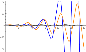
So we see the behavior of solutions depends on the value of parameter A: when it is greater than 1, solutions have different properties. Therefore, such value of A = 1 is called the bifurcation point (or node). Mathematica has a dedicated command NDSolve to find an a approximate solution to the initial value problem. Correspondingly, we use it to plot solutions of the given initial value problem for different values of parameter A.
sol1 = NDSolve[{x''[t] + (1/2 - Sin[2*t])*x[t] == 0, x[0] == 1, x'[0] == 0}, x, {t, 0, 30}, WorkingPrecision -> 24, InterpolationOrder -> All]
a1 = Plot[x[t] /. sol1, {t, 0, 30}, PlotStyle -> {Thick, Orange}]
sol = NDSolve[{x''[t] + (1 - Sin[2*t])*x[t] == 0, x[0] == 1, x'[0] == 0}, x, {t, 0, 30}, WorkingPrecision -> 24, InterpolationOrder -> All]
a2 = Plot[x[t] /. sol, {t, 0, 30}, PlotStyle -> {Thick, Blue}]
sol3 = NDSolve[{x''[t] + (2 - Sin[2*t])*x[t] == 0, x[0] == 1, x'[0] == 0}, x, {t, 0, 30}, WorkingPrecision -> 24, InterpolationOrder -> All]
a3 = Plot[x[t] /. sol3, {t, 0, 30}, PlotStyle -> {Thick, Black}]
Show[a1, a2, a3]

Solution for A = 1/2
   
Solution for A = 1
   
Solution for A = 2
   
All three solutions plotted together
When you give a setting for WorkingPrecision (which is an option for various numerical operations that specifies how many digits of precision should be maintained in internal computations), this typically defines an upper limit on the precision of the results from a computation. But within this constraint you can tell the Wolfram Language how much precision and accuracy you want to get. You should realize that for many kinds of numerical operations, increasing precision and accuracy goals by only a few digits can greatly increase the computation time required. Given a particular setting for WorkingPrecision, each of the functions for numerical operations in the Wolfram Language uses certain default settings for PrecisionGoal (which is an option for various numerical operations that specifies how many effective digits of precision should be sought in the final result) and AccuracyGoal (which is an option for various numerical operations which specifies how many effective digits of accuracy should be sought in the final result). Typical is the case of NDSolve, in which these default settings are equal to half the settings given for WorkingPrecision.

One can try to control the accuracy of numerical calculations by introducing the residual variable: \( z (t) = \ddot{x} = - \left( A - \sin 2t \right) x = \left( \sin 2t - A \right) x . \) Upon its differentiation, we get another system of differential equations with three unknowns:

\[ \begin{cases} \dot{x} =y , \\ \dot{y} = z , \\ \dot{z} = 2x\,\cos 2t + \left( \sin 2t - A \right) y , \end{cases} \qquad x(0) =1, \quad y(0) (0) =0 , \quad z(0) = -A. \]
This system of 3 differential equations is not equivalent to the original Mathieu equation because its general solution depends on 3 arbitrary constants and its existence requires a solution to be from the space C³. To eliminate extra constant, we need to impose the third initial condition, so the initial value problem will have the same solution as the original IVP for the Mathieu equation.

⁎ ✱ ✲ ✳ ✺ ✻ ✼ ✽ ❋


Now we generalize the previous examples by considering the general linear differential equation. Suppose we are given an n-th order linear differential equation

\begin{equation} \label{EqConv.5} x^{(n)} (t) + a_{n-1} x^{(n-1)} (t) + \cdots + a_1 x' (t) + a_0 x(t) = f(t) , \end{equation}
where all coefficients 𝑎i and function f are known. Upon introducing n new dependent variables
\[ y_1 (t) = x(t), \quad y_2 (t) = y'_1 (t) = x' (t), \quad y_3 (t) = y'_2 (t) = x'' (t), \quad \ldots , \quad y_n (t) = y'_{n-1} (t) = x^{(n-1)} (t) , \]
we reduce the given n-th order linear differential equation \eqref{EqConv.5} to an equivalent system of the first order equations.

We can assign to equation \eqref{EqConv.5} the differential operator \( L\left[ t, \texttt{D} \right] = \texttt{D}^n + a_{n-1} (t)\, \texttt{D}^{n-1} + \cdots + a_1 (t)\,\texttt{D} + a_0 (x)\,\texttt{I} , \) where \( \texttt{D} = {\text d}/{\text d}t \) and \( \texttt{D}^0 = \texttt{I} \) are the derivative operator and the identical operator, respectively. Then we rewrite the differential equation in a more concise form:

\[ L\left[ t, \texttt{D} \right] x(t) = f(t) . \]
When coefficients in this differential operator of order n do not depend on t, we obtain a constant coefficient differential operator \( L\left[ \texttt{D} \right] = \texttt{D}^n + a_{n-1} \, \texttt{D}^{n-1} + \cdots + a_1 \,\texttt{D} + a_0 \,\texttt{I}, \) to which we can assign a polynomial
\[ p(\lambda ) = \lambda^n + a_{n-1} \lambda^{n-1} + \cdots + a_1 \lambda + a_0 , \]
called the characteristic polynomial. Upon introducing n new dependent variables
\[ y_1 (t) = x(t), \quad y_2 = \dot{y}_1 , \quad y_3 = \ddot{y}_1 = \dot{y}_2 , \ldots , \quad y_{n} = \dot{y}_{n-1} , \]
we convert the given differential equation into the system of first order equations:
\[ \frac{\text d}{{\text d}t} \begin{bmatrix} y_1 \\ y_2 \\ \vdots \\ y_n \end{bmatrix} = {\bf C}_{p} \begin{bmatrix} y_1 \\ y_2 \\ \vdots \\ y_n \end{bmatrix} = \begin{bmatrix} 0 \\ 0 \\ \vdots \\ f(t) \end{bmatrix} . \]
where matrix
\begin{equation} \label{EqConv.6} {\bf C}_{p} = \begin{bmatrix} 0&1&0& \cdots &0&0 \\ 0&0&1& \cdots &0&0 \\ 0&0&0 \cdots &0&0 \\ \vdots&\vdots&\vdots& \ddots&\vdots&\vdots \\ 0&0&0& \cdots &0&1 \\ - a_0 & -a_1 & -a_2 & \cdots & -a_{n-2}& -a_{n-1} \end{bmatrix} \end{equation}
is called companion matrix for polynomial p(λ).
Theorem: For any polynomial p(λ), its companion matrix has the characteristic polynomial
\begin{equation} \label{EqConv.7} \chi (\lambda ) = \det \left( \lambda {\bf I} - {\bf C}_{p} \right) = p(\lambda ) \end{equation}
equal to the given polynomial.    ▣
Example 3: Consider a polynomial of the fourth degree \( p(\lambda ) = \lambda^4 + a\,\lambda^3 + b\, \lambda^2 + c\,\lambda + d , \) where d ≠ 0, and its companion matrix
\[ {\bf C}_4 = \begin{bmatrix} 0&1&0&0 \\ 0&0&1&0 \\ 0&0&0&1 \\ -d& -c& -b& -a \end{bmatrix} \qquad \Longrightarrow \qquad {\bf C}_4^{-1} = \begin{bmatrix} -c/d & -b/d & -a/d & -1/d \\ 1&0&0&0 \\ 0&1&0&0 \\ 0&0&1&0 \end{bmatrix} . \]
Inverse[{{0, 1, 0, 0}, {0, 0, 1, 0}, {0, 0, 0, 1}, {-d, -c, -b, -a}}]
{{-(c/d), -(b/d), -(a/d), -(1/d)}, {1, 0, 0, 0}, {0, 1, 0, 0}, {0, 0, 1, 0}}
Thus, the inverse of this companion matrix corresponds to the polynomial:
\[ \lambda^4 + \frac{c}{d}\, \lambda^3 + \frac{b}{d}\, \lambda^2 + \frac{a}{d}\, \lambda + \frac{1}{d} . \qquad \blacksquare \]

The same approach can be used to convert a nonlinear differential equation to an equivalent system of first order equations. It should be noted that nonlinear systems of differential equations can be solved only numerically (except for some rare cases). When a numerical solver is applied, it is common to introduce an auxiliary variable---the residual---in order to control accuracy. This approach is demonstrated in the following series of examples.

Example 4: Consider the initial value problem for the ideal pendulum equation
\[ \ddot{\theta} + \omega^2 \sin \theta =0 , \qquad \theta (0) = a = \frac{\pi}{3} \approx 1.0472 , \quad \dot{\theta} (0) = v = -\frac{1}{10}, \tag{4.1} \]
where the initial displacement 𝑎 and velocity v are specified, and ω² = (g/ℓ), with g being local acceleration due to gravity and ℓ being length of the rod containing a point mass. This equation is called the ideal pendulum equation because friction is not taken into account, the weight of the wire is neglected, and oscillation is assumed to be two-dimensional. When resistance is presented and assumed to be proportional to 
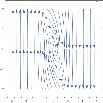
the velocity of the bob, the equation becomes
\[ \ddot{\theta} + k\,\dot{\theta} + \omega^2 \sin \theta =0 , \qquad \theta (0) = a , \quad \dot{\theta} (0) = v , \tag{4.2} \]
where k is a positive coefficient.

These problems (for ideal pendulum and pendulum with resistance) can be converted to equivalent systems of differential equations of the first order:

\[ \begin{cases} \dot{x} = y , \\ \dot{y} = - \omega^2 \sin x , \end{cases} \qquad x(0) =a, \quad y(0) = v ; \tag{4.3} \]
and
\[ \begin{cases} \dot{x} = y , \\ \dot{y} = - \omega^2 \sin x - k\,y , \end{cases} \qquad x(0) =a, \quad y(0) = v , \tag{4.4} \]
respectively. We plot its phase portraits using Mathematica:
LineIntegralConvolutionPlot[{{y, -Sin[x]}, {"noise", 1000, 1000}}, {x, -6, 6}, {y, -2, 2}, ColorFunction -> Hue, LightingAngle -> 0, LineIntegralConvolutionScale -> 3, Frame -> False]

   Phase portrait for undriven ideal pendulum
         
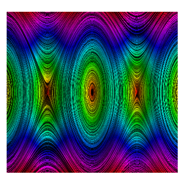
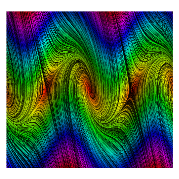
   Phase portrait for undriven pendulum with resistance


The ideal pendulum equation can be converted to a system of three equations upon introducing the residual variable:
\[ \begin{cases} \dot{x} = y , \\ \dot{y} = z , \\ \dot{z} = - \omega^2 y\,\cos x , \end{cases} \qquad x(0) =a, \quad y(0) = v , \quad z(0) = - \omega^2 \sin a . \]
So z is actually the second derivative of the original unknown function 
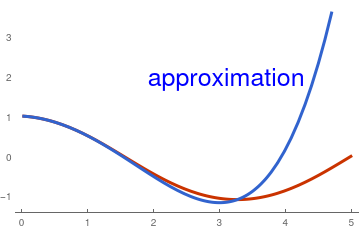
x(t). Therefore, the last equation is obtained by differentiation of the original pendulum equation with respect to time variable t. WE control approximation of the pendulum differential equation with the following Mathematica code:
      Since the function z(t) is supposed to be the second derivative, we can control the accuracy of Mathematica approximation of the pendulum equation by evaluating \( \ddot{\theta} + \sin \theta . \)
NDSolve[{x'[t] == y[t], y'[t] == z[t], z'[t] == -y[t]*Cos[x[t]], x[0] == Pi/3, y[0] == -1/10, z[0] == -Sin[Pi/3]}, {x, y, z}, {t, 0, 30}];
Plot[Evaluate[(z[t] + Sin[x[t]]) /. s], {t, 0, 10}, PlotRange -> All]
        Plot of \( \ddot{\theta} + \sin \theta . \)            Mathematica code

   ◾
Example 5: In the previous example, we converted the ideal pendulum equation \( \ddot{\theta} + \sin \theta =0 \) into the system of first order equations upon substituting y1 = θ and let y2 to be its derivative. Now we may define a new variable y3 = sinθ. According to the chain rule, its derivative is
\[ \frac{{\text d}y_3}{{\text d}t} = \left(\frac{{\text d}y_1}{{\text d}t} \right) \cos y_1 = y_2 \cos \theta . \]
Then we introduce a fourth dependent variable y4 = cosθ and obtain for it
\[ \frac{{\text d}y_4}{{\text d}t} = - \left(\frac{{\text d}y_1}{{\text d}t} \right) \sin y_1 = - y_2 \,y_3 . \]
Finally, we combine all equations together:
\begin{align*} \dot{y}_1 &= y_2 , \\ \dot{y}_2 &= -\omega^2 y_3 , \\ \dot{y}_3 &= y_2\, y_4 , \tag{5.1} \\ \dot{y}_4 &= -y_2\, y_3 . \end{align*}
The initial conditions for y3 and y4 will be related to those imposed on y1 and y2:
\[ y_1 (0) = a = \frac{\pi}{3}, \quad y_2 (0) = v = -\frac{1}{10}, \quad y_3 (0) = \sin a = \frac{\sqrt{3}}{2} \approx 0.866025, \quad y_4 (0) = \cos a = \frac{1}{2} . \tag{5.2} \]
Picard's iteration (see section in this tutorial) for this system of equations is
\[ {\bf \phi}_{m+1} (t) = \begin{bmatrix} y_1 (t) \\ y_2 (t) \\ y_3 (t) \\ y_4 (t) \end{bmatrix}_{(m+1)} = \begin{bmatrix} a \\ v \\ \sin a \\ \cos a \end{bmatrix} + \int_0^t {\text d}s \begin{bmatrix} y_2 (s) \\ - \omega^2 y_3 (s) \\ y_2 (s)\,y_4 (s) \\ -y_2 (s)\,y_3 (s) \end{bmatrix}_{(m)} , \qquad m= 0,1,2,\ldots . \tag{5.3} \]
Since the right-hand side in Eq.(5.3) is a polynomial, we can apply Picard's iteration. Performing a couple of iterations, we obtain
\[ \theta_{(3)} (t) = a + tv - \frac{t^2}{2}\, \sin a - \frac{t^3}{6}\,v\,\cos a . \]
a = Pi/3; v = -1/10;
s = NDSolve[{x''[t] + Sin[x[t]] == 0, x[0] == Pi/3, x'[0] == -1/10}, x, {t, 0, 20}];
phi0 = {a, v, Sqrt[3]/2, 1/2};
phi1[t_] = phi0 + t*{v, -w^2 *Sqrt[3]/2, v/2, -v*Sqrt[3]/2} phi2[t_] = phi0 + Integrate[{phi1[t][[2]], -w^2*phi1[t][[3]], phi1[t][[2]]*phi1[t][[4]], -phi1[t][[2]]*phi1[t][[3]]}, {t, 0, t}];
phi3[t_] = phi0 + Integrate[{phi2[t][[2]], -w^2*phi2[t][[3]], phi2[t][[2]]*phi2[t][[4]], -phi2[t][[2]]*phi2[t][[3]]}, {t, 0, t}];
phi4[t_] = phi0 + Integrate[{phi3[t][[2]], -w^2*phi3[t][[3]], phi3[t][[2]]*phi3[t][[4]], -phi3[t][[2]]*phi3[t][[3]]}, {t, 0, t}];
phi[t_] = Pi/3 - t/10 - (Sqrt[3] t^2)/4 + t^3/120 + ( 17 Sqrt[3] t^4)/1600 + t^5/800;
a + t v - 1/6 t^3 v Cos[a] - 1/2 t^2 Sin[a]
Now we plot the fourth approximation along with the true solution:
Plot[{Evaluate[x[t] /. s], phi[t]}, {t, 0, 5}, PlotTheme -> "Web", Epilog -> {Text[Style["approximation", 25, Blue], {3.1, 2}]}]
   ◾
Example 6: Consider the initial value problem for Duffing's equation
\[ \ddot{x} + k\,\dot{x} + x - \varepsilon\,x^3 = f(t) , \qquad x(0) =a, \quad \dot{x} = v , \tag{6.1} \]
where f(t) is a periodic forcing function, which can be chosen as \( f(t) = A\,\cos \omega t \) or \( f(t) = A\,\sin \omega t \) or their combination \( f(t) = A\,\sin \left( \omega t + \phi \right) . \) Here A is the amplitude, k is the dumping coefficient, and ε is a real number.

We convert it to the system of two differential equations

\[ \begin{cases} \dot{x} = y , \\ \dot{y} = - k\,y -x + \varepsilon\,x^3 + f(t) , \end{cases} \qquad x(0) =a, \quad y(0) = v . \tag{6.2} \]
Its direction field for undriven case is plotted with the following commands:
StreamPlot[{y, -y - x - x^3}, {x, -6, 6}, {y, -2, 2}, StreamScale -> Medium]
The residual system of equations becomes
\[ \begin{cases} \dot{x} = y , \\ \dot{y} = z , \\ \dot{z} = - k\,z - y - 3\varepsilon \, x^2 y - \dot{f} , \end{cases} \qquad x(0) =a, \quad y(0) = v , \quad z(0) = - k\,v - a - \varepsilon \, a^3 + f(0). \]
   ◾
Example 7: Consider a third order constant coefficient differential equation
\[ y''' +2\, y'' - y' -2 \,y = \sin (2t) . \tag{7.1} \]
Upon introducing three new dependent variables
\[ y_1 = y(t), \quad y_2 = \dot{y} = \dot{y}_1 , \quad y_3 = \ddot{y} = \dot{y}_2 , \tag{7.2} \]
we transfer the given single third order differential equation to the system of three equations of the first order
\begin{align*} \dot{y}_1 &= y_2 , \\ \dot{y}_2 &= y_3 , \tag{7.3} \\ \dot{y}_3 &= - 2\,y_3 + y_2 + 2\, y_1 + \sin (2t) . \end{align*}
We rewrite this system of equations in compact vector form:
\[ \frac{\text d}{{\text d}t} \begin{bmatrix} y_1 (t) \\ y_2 (t) \\ y_3 (t) \end{bmatrix} = \begin{bmatrix} 0&1&0 \\ 0&0&1 \\ -2& 1& 2 \end{bmatrix} \begin{bmatrix} y_1 (t) \\ y_2 (t) \\ y_3 (t) \end{bmatrix} + \begin{bmatrix} 0 \\ 0 \\ \sin (2t) \end{bmatrix} \tag{7.4} \]
The characteristic polynomial of the companion matrix
\[ \det \left( \lambda \begin{bmatrix} 1&0&0 \\ 0&1&0 \\ 0&0&1 \end{bmatrix} - \begin{bmatrix} 0&1&0 \\ 0&0&1 \\ 2&1&-2 \end{bmatrix} \right) = \lambda^3 + 2\,\lambda^2 - \lambda - 2\,\lambda = \left( \lambda^2 -1 \right) \left( \lambda +2 \right) \]
is in agreement with the characteristic polynomial for the given single differential equation.
A = {{0, 1, 0}, {0, 0, 1}, {-2, 1, 2}};
Eigenvalues[A]
{2, -1, 1}
CharacteristicPolynomial[A, s]
-2 + s + 2 s^2 - s^3
   ◾
Example 8: The Blasius equation for laminar flow over a flat plate can be reduced to the following differential equation of the third order:
\[ f''' + \frac{1}{2}\, f \, f'' =0 . \tag{8.1} \]
Upon introducing new functions:
\begin{eqnarray*} u_1 &=& f , \\ u_2 &=& f' = u'_1 , \\ u_3 &=& f'' = u'_2 , \end{eqnarray*}
we reduce the Blasius equation to a system of first order equations:
\[ \frac{{\text d}}{{\text d}y} \begin{bmatrix} u_1 \\ u_2 \\ u_3 \end{bmatrix} = \begin{bmatrix} u_2 \\ u_3 \\ - \frac{1}{2}\, u_1 u_2 \end{bmatrix} , \tag{8.2} \]
which is a nonlinear vector differential equation for three unknowns.


Classical Picard's iteration


In order to apply the classical Picard's iteration, we have to convert this to a system of first-order differential equations. Let

\[ f_1 = f, \qquad f_2 = f' , \qquad\mbox{and} \qquad f_3 = f'' . \]
This leads to:
\[ \frac{\text d}{{\text d}y} \begin{bmatrix} f_1 \\ f_2 \\ f_3 \end{bmatrix} = \begin{bmatrix} f_2 \\ f_3 \\ - \frac{1}{2}\, f_1 f_3 \end{bmatrix}, \qquad f_1 (0) =0, \quad f_2 (0) =0, \quad f_2 (\infty ) =1. \]
It is not possible to specify a boundary condition at ∞ numerically, so we will have to use a large number, and verify it is "large enough". From the solution, we evaluate the derivatives at y = 0, and we have f''(0) = f3(0).

We have to provide initial guesses for f1, f2 and f3. This is the hardest part about this problem. We know that f1 starts at zero, and is flat there (f'(0)=0), but at large y, it has a constant slope of one. We will guess a simple line of slope = 1 for f1. That is correct at large y, and is zero at y = 0. If the slope of the function is constant at large y, then the values of higher derivatives must tend to zero. We choose an exponential decay as a guess.

Finally, we let a solver iteratively find a solution for us, and find the answer we want.

We get the initial second derivative to be f''(0) = 0.3324911095517483. For the sake of simplicity, we approximate the Blasius constant as 1/3.

Now we use Picard iteration procedure starting with the initial conditions. Since the derivative operator is unbounded, we apply its inverse to reduce the given initial value problem into fixed point form:

\[ \frac{\text d}{{\text d}y} \begin{bmatrix} f_1 \\ f_2 \\ f_3 \end{bmatrix} = \begin{bmatrix} f_2 \\ f_3 \\ - \frac{1}{2}\, f_1 f_3 \end{bmatrix}, \qquad \begin{bmatrix} f_1 (0) \\ f_2 (0) \\ f_3 (0) \end{bmatrix} = \begin{bmatrix} 0 \\ 0 \\ 1/3 \end{bmatrix} \qquad \Longleftrightarrow \qquad \begin{bmatrix} f_1 (y) \\ f_2 (y) \\ f_3 (y)\end{bmatrix} = \begin{bmatrix} f_1 (0) \\ f_2 (0) \\ f_3 (0) \end{bmatrix} + \int_0^y \begin{bmatrix} f_2 (s) \\ f_3 (s) \\ - \frac{1}{2}\, f_1 (s)\,f_3 (s) \end{bmatrix} {\text d}s . \]
From this fixed point equation, we derive the iteration procedure
\[ \begin{bmatrix} f_{1,n+1} (y) \\ f_{2,n+1} (y) \\ f_{3,n+1} (y) \end{bmatrix} = \begin{bmatrix} 0 \\ 0 \\ 1/3 \end{bmatrix} + \int_0^y \begin{bmatrix} f_{2,n} (s) \\ f_{3, n} (s) \\ - \frac{1}{2}\, f_{1,n} (s)\,f_{3,n} (s) \end{bmatrix} {\text d}s , \qquad n=0,1,2,\ldots . \]
The initial approximation is just the initial conditions:
\[ \phi_{1,0} =0, \quad \phi_{2,0} =0, \quad \phi_{3,0} = 1/3 \quad\mbox{however, it should be the Blasius constant}. \]
The first iteration becomes
\[ \begin{bmatrix} \phi_{1,1} (y) \\ \phi_{2,1} (y) \\ \phi_{3,1} (y) \end{bmatrix} = \begin{bmatrix} 0 \\ 0 \\ 1/3 \end{bmatrix} + \int_0^y \begin{bmatrix} 0 \\ 1/3 \\ 0 \end{bmatrix} {\text d} y = \begin{bmatrix} 0 \\ y/3 \\ 1/3 \end{bmatrix} . \]
The second one is
\[ \begin{bmatrix} \phi_{1,2} (y) \\ \phi_{2,2} (y) \\ \phi_{3,2} (y) \end{bmatrix} = \begin{bmatrix} 0 \\ 0 \\ 1/3 \end{bmatrix} + \int_0^y \begin{bmatrix} y/3 \\ 1/3 \\ 0 \end{bmatrix} {\text d} y = \begin{bmatrix} y^2 /6 \\ y/3 \\ 1/3 \end{bmatrix} = \frac{1}{3} \begin{bmatrix} y^2 /2 \\ y \\ 1 \end{bmatrix} . \]
The third one is
\[ \begin{bmatrix} \phi_{1,3} (y) \\ \phi_{2,3} (y) \\ \phi_{3,3} (y) \end{bmatrix} = \begin{bmatrix} 0 \\ 0 \\ 1/3 \end{bmatrix} + \int_0^y \begin{bmatrix} y/3 \\ 1/3 \\ - y^2/36 \end{bmatrix} {\text d} y = \begin{bmatrix} y^2 /6 \\ y/3 \\ 1/3 - y^3/108 \end{bmatrix} = \frac{1}{3} \begin{bmatrix} y^2 /2 \\ y \\ 1 - y^3/36 \end{bmatrix} . \]
For next one, we have
\[ \begin{bmatrix} \phi_{1,4} (y) \\ \phi_{2,4} (y) \\ \phi_{3,4} (y) \end{bmatrix} = \begin{bmatrix} 0 \\ 0 \\ 1/3 \end{bmatrix} + \int_0^y \begin{bmatrix} y/3 \\ 1/3 - y^3/108 \\ - \frac{1}{36} \left( y^2 - \frac{y^5}{36} \right) \end{bmatrix} {\text d} y = \begin{bmatrix} y^2 /6 \\ \frac{y}{3} - \frac{y^4}{4 \cdot 108} \\ \frac{y^6}{36^3 \cdot 6} - \frac{y^3}{6\cdot 26} \end{bmatrix} = \frac{1}{3} \begin{bmatrix} y^2 /2 \\ y - \frac{y^4}{4 \cdot 36} \\ \frac{y^6}{2\cdot 36^2} - \frac{y^3}{36} \end{bmatrix} . \]
So our fifth approximation becomes
f1[y_] = y^2/6; f2[y_] = 1/3*(y - y^4/4/36); f3[y_] = 1/3*(y^6/2/36^2 - y^3 /36); f5[y_] = Simplify[Integrate[1/9*(s - s^4 /4/36), {s, 0, y}]]
-((y^2 (-360 + y^3))/6480)
\[ f_5 (y) = \frac{y^2}{6480} \left( 360 - y^3 \right) . \]
   ◾


Example 9: The generalized Genesio differential equation is of the form
\[ \dddot{x} + a\,\ddot{x} + b\,\dot{x} + c\,x + h(x) = 0 , \]
where \( \displaystyle h(x) = \sum_{k=1}^n (-1)^k x^{2k} \) and 𝑎, b, and c are arbitrary real parameters. We consider a simple version of the Genesio equation when chaotic jerk is observed:
\[ \dddot{x} + \dot{x} - x^2 + x^4 = 0 , \tag{9.1} \]
Upon introducing new functions:
\begin{eqnarray*} x_1 &=& x , \\ x_2 &=& x' = x'_1 , \\ x_3 &=& x'' = x'_2 , \end{eqnarray*}
we reduce the Genesio equation to a system of first order equations:
\[ \frac{{\text d}}{{\text d}t} \begin{bmatrix} x_1 \\ x_2 \\ x_3 \end{bmatrix} = \begin{bmatrix} x_2 \\ x_3 \\ - x_2 + x_1^2 - x_1^4 , \end{bmatrix} , \tag{9.2} \]
which is a nonlinear vector differential equation for three unknowns.
      We make a numerical experiment and plot two solutions of the Genesio equation for small values of parameters 𝑎 = 0.1 and c = 0.1, and then compare with the case when they are zero.
sol3 = NDSolve[{x'''[t] + 1*x'[t] - (x[t])^2 + (x[t])^4 == 0, x[0] == 1, x'[0] == -0.1, x''[0] == 0}, x, {t, 0, 3}];
sol3a = NDSolve[{x'''[t] + 0.1*x''[t] + 1*x'[t] + 0.1*x[t] - (x[t])^2 + (x[t])^4 == 0, x[0] == 1, x'[0] == -0.1, x''[0] == 0}, x, {t, 0, 3}];
Plot[{Evaluate[x[t] /. sol3], Evaluate[x[t] /. sol3a]}, {t, 0, 3}, PlotTheme -> "Marketing"]
       Two solutions of the Genesio equation.            Mathematica code

   ◾
  1. Brand, L., The companion matrix and its properties, The American Mathematical Monthly, 1964, Vol. 71, No. 6, pp. 629--634.
  2. Eastham, M.S.P., "The spectral theory of periodic differential equations" , Scottish Acad. Press (1973)
  3. Hill, G. W. "On the Part of the Motion of Lunar Perigee Which is a Function of the Mean Motions of the Sun and Moon." Acta Math. 8, 1-36, 1886.
  4. Magnus,W., Winkler, S., "Hill's equation" , Dover, reprint (1979)
  5. V.A. Yakubovich, V.M. Starzhinskii, "Linear differential equations with periodic coefficients" , Wiley (1975) (Translated from Russian)


Return to Mathematica page
Return to the main page (APMA0340)
Return to the Part 1 Matrix Algebra
Return to the Part 2 Linear Systems of Ordinary Differential Equations
Return to the Part 3 Non-linear Systems of Ordinary Differential Equations
Return to the Part 4 Numerical Methods
Return to the Part 5 Fourier Series
Return to the Part 6 Partial Differential Equations
Return to the Part 7 Special Functions