Preface
The following sections are devoted to Laplace and Helmholtz equations as typical representatives of the elliptic partial differential equations. We mostly deal with the plane case when the number of independent variables is restricted to be two. However, some three dimensional cases are also included in the tutorial. Elliptic differential equations occur in many applications; its theory contains many important results of which only few are included.
Return to computing page for the first course APMA0330
Return to computing page for the second course APMA0340
Return to Mathematica tutorial for the first course APMA0330
Return to Mathematica tutorial for the second course APMA0340
Return to the main page for the first course APMA0330
Return to the main page for the second course APMA0340
Return to Part VI of the course APMA0340
Introduction to Linear Algebra with Mathematica
Glossary
Elliptic Equations
Let A(x,y), B(x,y), and C(x,y) be known differentiable functions in some domain Ω ⊂ ℝ² with smooth boundary ∂Ω. The differential operator of second order
Typical examples of elliptic equations give famous Laplace's equation
This principle can be generalized for arbitrary elliptic operator,
Example: Consider the Helmholtz equation (42, page 76) \[ u_{xx} + u_{yy} + 2u = 0 \qquad (0 < x < \pi , \quad 0 < y < \pi ). \tag{Helmholtz.1} \] Then the function u = u(x, y) = sin(x) sin(y) is a solution of Eq.(Helmholtz.1) in the square S = [0, π} × [0, π] and vanish on the perimiter of S without vanishing inside S. ■
Example: Consider the Helmholtz equation (42, page 184) \[ u_{xx} + u_{yy} - 4u = 0 \qquad (-\infty < x < \infty , \quad 0 < y < \infty ). \tag{Helmholtz.2} \] in half plane \[ \Omega : \quad y \ge 0 \quad \mbox{and} \quad x \in \mathbb{R} = (-\infty , \infty ). \] Eq.(Helmholtz.2) has a regular solution in Ω that vanish on the boundary ∂Ω : y = 0 and x ∈ ℝ without identically vanishing in Ω.
In gact, such a solution is of the form \[ u = u(x,y) = \sinh \left( x \sqrt{2} \right) \sinh \left( y \sqrt{2} \right) . \] ■
Example: Consider the Laplace equation \eqref{EqElliptic.1} \( u_{xx} + u_{yy} = 0 \) in the unbounded domain (16, page 20) \[ \Omega = \left\{ (x,y) \in \mathbb{R}^2 \,: \ -\infty < x < \infty , \quad 0 < y < \pi \right\} . \] This Laplace equation has regular solution \[ u = u(x,y) = e^x \,\sin y \] in Ω that vanishes on the boundary ∂Ω : y = 0 and y = π, −∞ < x < ∞, without identically vanishing in Ω. ■
This formula can be generalized for arbitrary self-adjoint elliptic operator \( L[u] = \mbox{div}\left( k\,\nabla \,u \right) - q\, u \) and for biharmonic operator.
Dirichlet's boundary conditions or boundary conditions of the first kind:
Third kind boundary conditions (that are also frequently called mixed):
When we consider heat transfer problems, the Dirichlet boundary conditions correspond to prescribing temperature on the boundary. The Neumann boundary conditions correspond to prescribing heat flux on the boundary. The convective boundary conditions leads to the third kind boundary conditions. An elliptic partial differential equation with one of corresponding boundary conditions is called the boundary value problem. Out of these, there are two important classes of boundary value problems: interior or inner boundary value problems and exterior or outer boundary value problems. They are ussually referred to a finite domain Ω ⊂ ℝn and a solution is seeking either inside Ω or outside it.
There are two main reasons for considering these three kinds of boundary conditions. First, they are mostly used in practical applications; and second, the corresponding boundary value problems have solutions. These boundary value problems also have unique solutions except Neumann's conditions. On the plane (the number of independent variables is 2), the Neumann boundary value problem for the Laplace equation is determined up to arbitrary additive constant. Moreover, the boundary function f(x,y) should also satisfy some auxiliary condition for existence of the solution. In multi-dimensional case, the situation is slightly different, but still requires some additional conditions. All these statements are valid only when the boundary ∂Ω of the finite domain Ω is smooth. When the boundary has singular points where its curve/surface is not differentiable (we call such points wedge or corner points), then the given boundary value problem may have multiple solution, and additional conditions must be imposed to guarantee its uniqueness. On the plane, it is required that the solution should be bounded when a point approaches the corner. Such condition is called the wedge condition. In arbitrary n-dimensional case (when n ≥ 3), these conditions will be different from the plane case. In general, the lack of boundary regularity or the transmission conditions result in singular behavior of the solution near such point. The boundary value problems with singular points on the boundary were studied extensively. A thorough survey can be found in Kondrat'ev--Oleinik papers. When tangent lines from both sides of the corner point coincide (as for instance in the heart shape domain ❤), the boundary value problem has no solution.
Consider a domain \( \Omega \subset \mathbb{R}^n \) in n dimensional space, and a function \( u\,:\, \overline{\Omega} \to \mathbb{R} \) defined on Ω and its boundary. We assume that the boundary \( \partial\Omega \) of the domain and the function are sufficiently smooth. In particular, the boundary should not have corner points---this case will be analyzed separately.
The Dirichlet integral (functional) of u over Ω is defined by
Let \( h\,:\,\overline{\Omega} \to \mathbb{R} \) be a smooth function that satisfies either homogeneous Dirichlet boundary condition \( \left. u \right\vert_{\partial \Omega} =0 \) or homogeneous Neumann condition \( \left. \partial u/\partial{\bf n} \right\vert_{\partial \Omega} =0 . \) Since the further derivations only slightly differ from each other in the case of Dirichlet boundary condition and the Neumann boundary condition, we consider for simplicity only the latter one. Calculation of the variational derivative of the Dirichlet functional yields
|
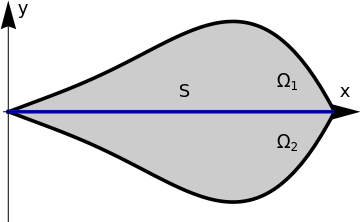
Consider a domain Ω consisting of two adjacent domains Ω1 and Ω2, separated by set S (see Figure 1), so that
\[
\Omega = \Omega_1 \cup \Omega_2 \cup S .
\]
Assume that the closure of S is a surface of class C¹.
(42, pages 235--237).
domain = Plot[{x^{1/20}*(2*Pi - x)*Sin[x/2]/15 +
x^2*Sin[x/2]/20, -x^{1/20}*(2*Pi - x)*Sin[x/2]/15 -
x^2*Sin[x/2]/20}, {x, 0, 2*Pi},
PlotRange -> {{-0.15, 2*Pi + 0.5}, {-1.1, 1.1}}, Axes -> False,
PlotStyle -> {{Thickness[0.01], Black}, {Thickness[0.01], Black}},
Filling -> {1 -> {2}}];
line = Plot[0, {x, 0, 2*Pi}, PlotStyle -> {Thickness[0.01], Blue}, Axes -> False]; ar1 = Graphics[{Black, Arrowheads[0.08], Arrow[{{-0.1, 0}, {2*Pi + 0.5, 0}}]}]; ar2 = Graphics[{Black, Arrowheads[0.08], Arrow[{{0, -1.1}, {0, 1.1}}]}]; t1 = Graphics[ Text[Style[ ToString[Subscript[\[CapitalOmega], 1], TraditionalForm], FontSize -> 18], {5.4, 0.3}]]; t2 = Graphics[ Text[Style[ ToString[Subscript[\[CapitalOmega], 2], TraditionalForm], FontSize -> 18], {5.4, -0.3}]]; s = Graphics[ Text[Style[ToString["S", TraditionalForm], FontSize -> 18], {3.4, 0.2}]]; x = Graphics[ Text[Style[ToString["x", TraditionalForm], FontSize -> 18], {6.5, 0.2}]]; y = Graphics[ Text[Style[ToString["y", TraditionalForm], FontSize -> 18], {0.3, 1.02}]]; Show[domain, line, ar1, ar2, t1, t2, s, x, y] |
|
| Domain Ω = Ω1 ∪ Ω2 ∪ S. | Mathematica code |
Example: Let S = (0, 1) be the interval on the abscissa and Ω1 = y > 0; correspondingly, Ω2 = y < 0. Let u(x, y) satisfies Laplace's equation uxx + uyy = 0 and the initial conditions
- Elliptic problems on polyhedral domains, TAMU.
- Grisvard, P.: Elliptic problems in non-smooth domains. London: Pitman 1985
- Karl Gustafson and Takehisa Abe. The third boundary condition—was it robin’s? The Mathematical Intelligencer, March 1998, Volume 20, Issue 1, pp 63--71.
- Kondratiev, V.A., Boundary value problems for elliptic equations in domains with conical or angular points, Transactions of the Moscow Mathematical Society, 1967, Vol. 16, 227--313.
- Kondrat'ev, V.A., Oleinik, O.A.: Boundary-value problems for partial differential equations in non-smooth domains. Russian Mathematical Survey, 1983, Vol. 38, No. 2, pp. 1–86.
- Moon, P., and Spencer, D.~E., The meaning of the vector Laplacian, Journal of The Franklin Institute, 1953, 256, Issue 6, 551--558.
- Schechter, M., General boundary value problems for elliptic partial differential equations, Bulletine of the American Mathethatical Society, 1959, Volume 65, Number 2, pp. 70--72.
- Serkh, K. and Rokhlin, V., On the solution of the Helmholtz equation on regions with corners, Proceedings of the National Academy of Sciences of the United States of America, 2016, Vol. 113, pp. 9171--9176. https://doi.org/10.1073/pnas.1609578113
- Spence, E.A., Boundary Value Problems for Linear Elliptic PDEs, 2009, Dissertation, Cambridge.
- Zhevandrov, P. and Merzon, A., On the Neumann problem for the Helmholtz equation in a plane angle, Journal of Applied Mathematics and Mechanics, 2000, Vol. 23, pp. 1401--1446.
Return to Mathematica page
Return to the main page (APMA0340)
Return to the Part 1 Matrix Algebra
Return to the Part 2 Linear Systems of Ordinary Differential Equations
Return to the Part 3 Non-linear Systems of Ordinary Differential Equations
Return to the Part 4 Numerical Methods
Return to the Part 5 Fourier Series
Return to the Part 6 Partial Differential Equations
Return to the Part 7 Special Functions