Return to computing page for the first course APMA0330
Return to computing page for the second course APMA0340
Return to Mathematica tutorial for the first course APMA0330
Return to Mathematica tutorial for the second course APMA0340
Return to the main page for the course APMA0340
Return to the main page for the course APMA0330
Introduction to Linear Algebra with Mathematica
This section is a collection of Fourier series expansions for different step functions. Square wave function constitute a very important class of functions used in electrical engineering and computer science; in particular, in music synthesizors. A square wave function, also called a pulse wave, is a periodic waveform consisting of instantaneous transitions between two levels. We consider two cases of square waves that include the digital signal (0,1) and oscillation between (-1,1). Other common levels for the square wave includes -½ and ½.
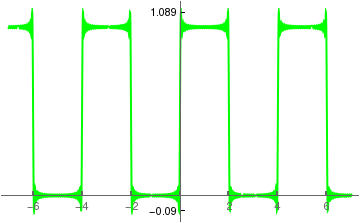
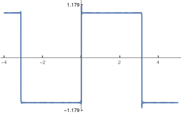
We start with the Heaviside function on finite interval [-2,2], which we extend in periodic manner with period 4:
Integrate[Cos[n*Pi*x/a], {x,0,a}]/a
There is no need to show Mathematica commands for Fourier coefficient evaluations---it was done in the previous sections. However, for completeness, we evaluate Fourier coefficients.
We can also expand the Heaviside function into Fourier sine and Fourier cosine series on the interval [0,2ℓ]. To achieve this, we expand the Heaviside function evenly and oddly from the given interval:
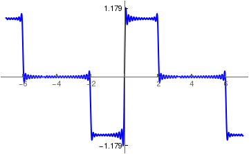
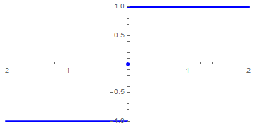
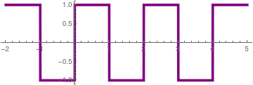
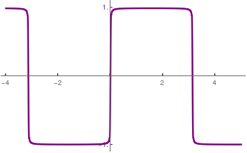
In order to expand the signum function into the Fourier series, we need to choose a value ℓ and expand this function in odd way periodically from the interval (−&wll;, ℓ).
We expect that the Fourier series will give a periodic expansion shown in the figure.
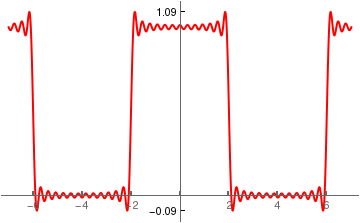
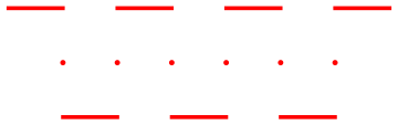
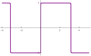
g[x_] = Piecewise[{{1, 0 < x < 1}, {-1,
1 < x < 2}, {-1, -1 < x < 0}, {1, -2 < x < -1}, {1,
2 < x < 3}, {-1, 3 < x < 4}, {1, 4 < x < 5}}];
sign = Plot[g[x], {x, -2, 5}, PlotStyle -> {Thickness[0.01], Red},
AspectRatio -> 1/3];
point = Graphics[{Red, {Disk[{-1, 0}, 0.05], Disk[{0, 0}, 0.05],
Disk[{1, 0}, 0.05], Disk[{2, 0}, 0.05], Disk[{3, 0}, 0.05],
Disk[{4, 0}, 0.05]}}];
Show[point, sign]
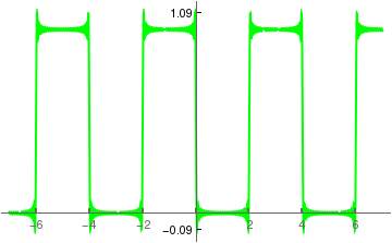
However, if you want remove the point valuse on the horizontal axis, you can include plot option Exclusions → None.
We plot oddsign function without dots:
g[x_] = Piecewise[{{1, 0 < x < 1}, {-1,
1 < x < 2}, {-1, -1 < x < 0}, {1, -2 < x < -1}, {1,
2 < x < 3}, {-1, 3 < x < 4}, {1, 4 < x < 5}}];
Plot[g[x], {x, -2, 5}, PlotStyle -> {Thickness[0.01],Purple},
AspectRatio -> 1/3, Exclusions -> None]
As a result, we obtain the periodic version of the signum function that we denote as oddsign; its sine Fourier series is
Since this function is odd, there is no difference between its Fourier series and Fourier sine series; that is why we plot it in blue. Next, we calculate its Fourier coefficients:
You can use instead the build-in Mathematica commands: FourierSinCoefficient[Sign[x], x, n, FourierParameters -> {1,(π)/L}] FourierCosCoefficient[Sign[x], x, n, FourierParameters -> {1,(π)/L}]
For ℓ = π, we get
FourierSinCoefficient[Sign[x], x, n, FourierParameters -> {1, 1}]
-((2 (-1 + (-1)^n))/(n \[Pi]))
We can also expand the signum function into complex Fourier series:
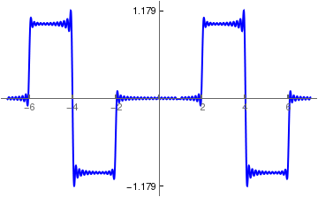
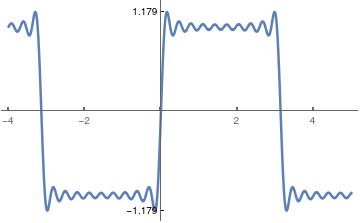
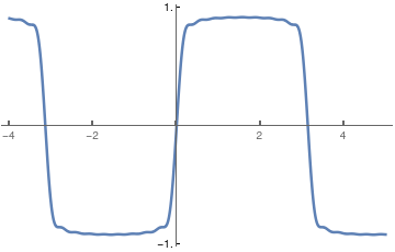
Of course, this series is exactly the same as (1.3). Our next step is to truncate the series (1.3) or (1.4) and show how the finite Fourier series converges to the signum function. First, we use animation:
We plot partial sums with n = 10, 100, and 1000 terms.
Its Fourier series exhibits the Gibbs phenomenon at points of discontinuity x = (2n+1)ℓ, n∈ℤ, in amount of 2w ≈ 0.1789797, where w = 0.5707963267948966 is the Wilbraham number (see section). Recall that the value of the overshoot or undershoot of the partial Fourier sum is equal to h w, where h is the jump of discontinuoity (which 2 in our case).
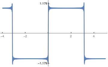
It is known that restoring a function from its Fourier coefficients is an ill-posed problem. The Gibbs phenomenon clearly indicates that it is impossible to recover the function in a neighbohood of the point of discontinuity. A wealth of information hidden in the Fourier series can be recovered upon utilization of a summability method.
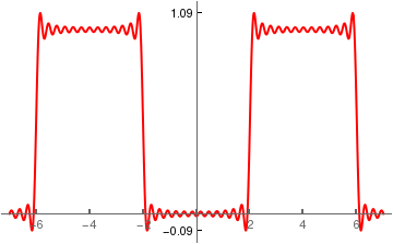
For practical applications, its regularization, can be obtained with Cesàro's summation:
Note that Cesàro's regularization requires only three additional arithmetic operations on each step compared with the standard summation: one multiplication by the difference (1−k/n), one division (k/n), and one subtraction. This usually does not increase the time of computation.
Finally, we demonstrate animation for Cesàro's approximation
Now we demonstrate how Fourier approximation depends on the number of terms (graphs present 3 terms, 7 terms, 10 terms, and 20 terms, but you can choose any numbers instead).
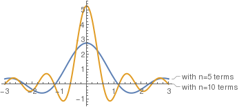
Since the delta-function is a distribution but not a regular function, the series above cannot truly converge (its terms don’t approach zero). But we can determine its partial sums and graph the latter. We naturally denote such partial sums by
This is a geometric progression that starts from \( e^{-N{\bf j}\theta} \) and ends at \( e^{N{\bf j}\theta} . \) We have powers of the same exponential factor \( e^{{\bf j}\theta} . \) The sum of a geometric series is known:
\[
\delta_N (x) = \frac{1}{2\ell} \, \frac{e^{{\bf j} (N+ 1/2) \pi x /\ell} - e^{-{\bf j} (N+ 1/2) \pi x /\ell}}{e^{{\bf j}\pi x /\ell} - e^{-{\bf j}\pi x /\ell}} = \frac{1}{2\ell} \, \frac{\sin (N+1/2) x/\ell}{\sin (x/2/\ell)}
\]
This partial sum approaches the Dirac delta-function in weak sense, so for any smooth probe function f, we expect
The graph of each δh(x) is a tall thin rectangle: height
1/h, base h, and area=1. When h approaches zero, δh(x) is squeezed into a very thin interval. The tall
rectangle approaches (weakly) the delta function δ(x). The Fourier coefficients of δh(x) are
Return to the main page (APMA0340)
Return to the Part 1 Matrix Algebra
Return to the Part 2 Linear Systems of Ordinary Differential Equations
Return to the Part 3 Non-linear Systems of Ordinary Differential Equations
Return to the Part 4 Numerical Methods
Return to the Part 5 Fourier Series
Return to the Part 6 Partial Differential Equations
Return to the Part 7 Special Functions