Preface
Not every solution to the Duffing equation is bounded---it depends on the initial conditions and pareametrers of the input periodic function.
Forced anharmonic motion
Our main concern is the existence of bounded solutions to the forced Duffing equation
\begin{equation} \label{EqDuffing.1}
x'' + x(t) - \frac{1}{6}\, x^3 = F\,\cos \left( \omega\,t \right) , \qquad x(0) = a, \quad x' (0) = b .
\end{equation}
We are going to numerically investigate the dependence of existence of bounded solutions on the values of parameters of this Duffing equation. It turns out that the bounded solution exists for some values of parameters and it has unbounded solutions for other parameter values. We break these parameters into two groups, and consider fest dependence of solution on the initial values (𝑎, b) and then on the values of input parameters (F, ω)
Dependence on initial conditions
\begin{equation} \label{EqDuffing.2}
x'' + x(t) - \frac{1}{6}\, x^3 =0.3\,\cos \left( 0.5\,t \right) , \qquad x(0) = a, \quad x' (0) = b .
\end{equation}
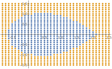
Not for arbitrary values of initial parameters (𝑎,b) the given initial value problem has a bounded solution. So we check with Mathematica.
|
pfun = ParametricNDSolveValue[{x''[t] == -x[t] + x[t]^3/6 +
0.3*Cos[0.5*t], x[0] == a, x'[0] == b}, x, {t, 0, 100}, {a, b}];
allPars = Flatten[Chop[ Table[{a, b}, {a, -0.8, 2.5, 0.1}, {b, -1.5, 1.5, 0.1}]], {1, 2}];; validPars = {}; invalidPars = {}; Table[If[Apply[pfun, par]["Domain"] === {{0.`, 100.`}}, AppendTo[validPars, par], AppendTo[invalidPars, par]], {par, allPars}]; ListPlot[{validPars, invalidPars}, PlotLegends -> {"Valid Parameters", "Invalid Parameters"}, PlotStyle -> {Directive[PointSize[0.015]]}] |
|
| Region of bounded solutions | Mathematica code |
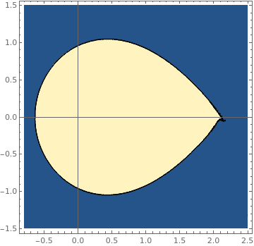
There is another approach:
|
fun1[a_?NumericQ, b_?NumericQ] := Module[
{res},
(* determine if domain is valid or invalid and return 1 or 0 respectively *) res = Quiet[pfun[a, b]]; Boole[res["Domain"] === {{0., 100.}}]; ]; ContourPlot[fun1[a, b], {a, -0.8, 2.5}, {b, -1.5, 1.5}, PlotPoints -> 50, MaxRecursion -> 3, Axes -> True, AxesOrigin -> {0, 0}] |
|
| Region of bounded solutions | Mathematica code |
|
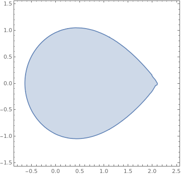
We make a region using the boolean function defined earlier
regionplot = RegionPlot[fun[a, b] >= 1, {a, -0.6, 2}, {b, -1, 1}]
|
|
| Region of bounded solutions | Mathematica code |
|
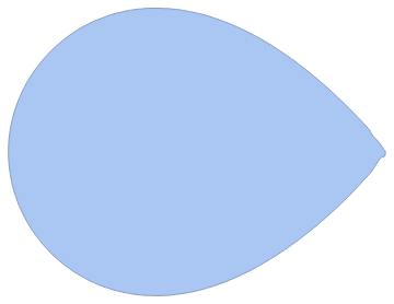
Create a boundary mesh from the region
mesh = BoundaryDiscretizeGraphics[regionplot]
|
|
| Boundary of the domain | Mathematica code |
|
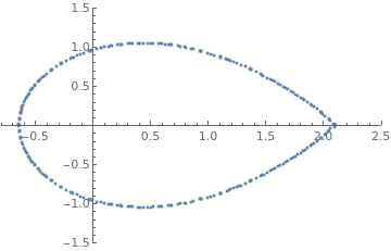
Now we generate the set of coordinates; however, they are not ordered. As you increase n using the slider, the curve fills up in random spots
Manipulate[
ListPlot[coord[[1 ;; n]], PlotRange -> {{-0.8, 2.5}, {-1.5, 1.5}}],
{{n, 50}, 1, Length[coord], 1}
]
|
|
| Boundary of the region | Mathematica code |
Next we sort the boundary coordinates.
MeshCells[] will give the lines that connect different points. Note that the arguments for Line[] are the coordinate indices (not the coordinate positions)
meshLines = MeshCells[mesh, 1];
meshLines // Short
{Line[{1,2}], Line[{2,42}], Line[{42.40}], >>272<<, Line[{122,123}], Line[{123,1}]}
Get the order of points
orderOfPoints = (Apply[Sequence, #] & /@ meshLines)[[All, 1]];
orderOfPoints // Short
{1, 2, 42, 41, 221, 92,34, 35, 36, 37, >>252<<, 27, 275, 214, 215, 229, 230, 217, 218, 157, 122, 123}
Sort the coordinates we obtained earlier
sortedcoord = coord[[orderOfPoints]];
The points are then further ordered so we start at the right end of the shape (this is optional)
While[sortedcoord[[1, 1]] != Max[sortedcoord[[All, 1]]],
sortedcoord = RotateLeft[sortedcoord, 1]; ]
|
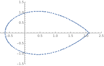
Use the slider below to see that the points are now ordered
Manipulate[
ListPlot[sortedcoord[[1 ;; n]],
PlotRange -> {{-0.8, 2.5}, {-1.5, 1.5}}],
{{n, 50}, 1, Length[sortedcoord], 1}
]
|
|
| The boundary of the domain, | Mathematica code |
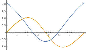
Parametrizing the x- and y- coordinates separately in terms of pairs. Find the distance between each successive pair of points, and then the distances are added up cumulatively using
Accumulate[] (this will be the parameter for the x- and y- coordinates).
dist = Accumulate[Prepend[Norm /@ Differences[sortedcoord], 0.]];
Building the list of points {{p1, x1}, {p2, x2}.. {pn, xn}} and {{p1, y1}, {p2, y2}.. {pn, yn}} and fitting with an interpolation function.
|
{px, py} = Transpose[{dist, #}] & /@ Transpose[sortedcoord];
{funca, funcb} = Interpolation[#, InterpolationOrder -> 1] & /@ {px, py}; Show[ Plot[{funca[p], funcb[p]}, {p, 0, dist[[-1]]}], ListPlot[{px, py}, PlotLegends -> {"\!\(\*SubscriptBox[\(p\), \ \(i\)]\),\!\(\*SubscriptBox[\(x\), \(i\)]\)", "\!\(\*SubscriptBox[\(p\), \(i\)]\),\!\(\*SubscriptBox[\(y\), \(i\ \)]\)"}] ] |
|
|
Plot of the boundary coordinates separately. |
Mathematica code |
|
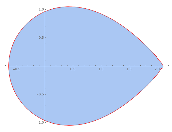
See the parametric plot of the interpolation function and compare to the region
Show[
ParametricPlot[{funca[p], funcb[p]}, {p, 0, dist[[-1]]},
PlotStyle -> {Thickness[0.005], Red}, ImageSize -> Large],
mesh
]
|
|
| The boundary of the domain, | Mathematica code |
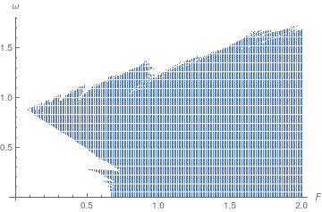
Dependence on input values
\begin{equation} \label{EqDuffing.3}
x'' + x(t) - \frac{1}{6}\, x^3 = F\,\cos \left( \omega\,t \right) , \qquad x(0) = 0, \quad x' (0) = 0 .
\end{equation}
divergentValues =
Reap[Table[
Check[NDSolveValue[{x''[t] + x[t] - (1/6)*(x[t])^3 ==
F*Cos[omega*t], x[0] == 0, x'[0] == 0}, x, {t, 0, 100}],
Sow[{F, omega}]], {F, .01, 2, .01}, {omega, 0, 3, .01}];][[2]];
ListPlot[divergentValues, AxesLabel -> {F, \[Omega]}]
ListPlot[divergentValues, AxesLabel -> {F, \[Omega]}]
(* F = 1 *)
s = NDSolve[{x''[t]== -x[t] - x[t]^3 + 1*Cos[t], x[0]==1, x'[0]==0},x,{t,0,100}]
ParametricPlot[Evaluate[{x[t],x'[t]}/.s],{t,0,100}]
(* F = 1.5 *)
s2 = NDSolve[{x''[t]== -x[t] - x[t]^3 + 1.5*Cos[t], x[0]==1, x'[0]==0},x,{t,0,100}]
ParametricPlot[Evaluate[{x[t],x'[t]}/.s2],{t,0,100}]
(* F = 2.1 *)
s3 = NDSolve[{x''[t]== -x[t] - x[t]^3 + 2.1*Cos[t], x[0]==1, x'[0]==0},x,{t,0,100}]
ParametricPlot[Evaluate[{x[t],x'[t]}/.s3],{t,0,100}]
(* F = 3 *)
s4 = NDSolve[{x''[t]== -x[t] - x[t]^3 + 3*Cos[t], x[0]==1, x'[0]==0},x,{t,0,100}]
ParametricPlot[Evaluate[{x[t],x'[t]}/.s4],{t,0,100}]
(* omega = 2 *)
(* F = 1 *)
w = NDSolve[{x''[t]== -x[t] - x[t]^3 + 1*Cos[2*t], x[0]==1, x'[0]==0},x,{t,0,100}]
ParametricPlot[Evaluate[{x[t],x'[t]}/.w],{t,0,100}]
(* F = 0.5 *)
w2 = NDSolve[{x''[t]== -x[t] - x[t]^3 + 0.5*Cos[2*t], x[0]==1, x'[0]==0},x,{t,0,100}]
ParametricPlot[Evaluate[{x[t],x'[t]}/.w2],{t,0,100}]
(* F = 4.3 *)
w3 = NDSolve[{x''[t]== -x[t] - x[t]^3 + 4.3*Cos[2*t], x[0]==1, x'[0]==0},x,{t,0,100}]
ParametricPlot[Evaluate[{x[t],x'[t]}/.w3],{t,0,100}]
(* F = 5 *)
w4 = NDSolve[{x''[t]== -x[t] - x[t]^3 + 5*Cos[2*t], x[0]==1, x'[0]==0},x,{t,0,100}]
ParametricPlot[Evaluate[{x[t],x'[t]}/.w4],{t,0,100}]
- Hasting, C., Mischo, K., Morrison, M., Hands-on start to Wolftam Mathematica, 2020, third edition, WolframMedia.
Return to Mathematica page
Return to the main page (APMA0340)
Return to the Part 1 Matrix Algebra
Return to the Part 2 Linear Systems of Ordinary Differential Equations
Return to the Part 3 Non-linear Systems of Ordinary Differential Equations
Return to the Part 4 Numerical Methods
Return to the Part 5 Fourier Series
Return to the Part 6 Partial Differential Equations
Return to the Part 7 Special Functions