Preface


This tutorial was made solely for the purpose of education and it was designed for students taking Applied Math 0340. It is primarily for students who have some experience using Mathematica. If you have never used Mathematica before and would like to learn more of the basics for this computer algebra system, it is strongly recommended looking at the APMA 0330 tutorial. As a friendly reminder, don't forget to clear variables in use and/or the kernel. The Mathematica commands in this tutorial are all written in bold black font, while Mathematica output is in regular fonts.

Finally, you can copy and paste all commands into your Mathematica notebook, change the parameters, and run them because the tutorial is under the terms of the GNU General Public License (GPL). You, as the user, are free to use the scripts for your needs to learn the Mathematica program, and have the right to distribute and refer to this tutorial, as long as this tutorial is accredited appropriately. The tutorial accompanies the textbook Applied Differential Equations. The Primary Course by Vladimir Dobrushkin, CRC Press, 2015; http://www.crcpress.com/product/isbn/9781439851043

Return to computing page for the first course APMA0330
Return to computing page for the second course APMA0340
Return to Mathematica tutorial for the first course APMA0330
Return to Mathematica tutorial for the second course APMA0340
Return to the main page for the first course APMA0330
Return to the main page for the second course APMA0340
Return to Part VI of the course APMA0340
Introduction to Linear Algebra

Laplace equation in a wedge


Recall that both the real and imaginary parts of an analytic function satisfy 
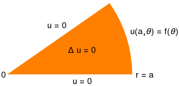
Laplace’s equation in two dimension. Suppose the region of interest is defined by the angular wedge W = 0 ≤ θ ≤ α. Consider the analytic function
\[ f(z) = z^{\pi /\alpha} = r^{\pi /\alpha} \left( \cos \frac{\pi\theta}{\alpha} + {\bf j}\,\sin \frac{\pi\theta}{\alpha} \right) , \]
of which we consider the principal branch. If α = π/m for some integer m, then f(z) is analytic everywhere. If α is an arbitrary real number, then f(z) may have a branch point at the origin, but we may choose the branch cut so that f(z) is still analytic in our region everywhere except at the origin. In fact the function \( f_n (z) = z^{n\pi /\alpha} \) for any integer n has the same nice properties. Then its real part \( u(t, \theta ) = \Re f(z) = r^{\pi /\alpha} \cos \frac{\pi\theta}{\alpha} \) and imaginary part \( v(t, \theta ) = \Im f(z) = r^{\pi /\alpha} \sin \frac{\pi\theta}{\alpha} \) are both solutions of the Laplace's equation:
\[ \Delta u =0 \qquad\mbox{and}\qquad \Delta v =0 \]
in the wedge. Thus, the potential in a wedge-shaped region W with opening angle α and conducting boundaries at potential V0 is described by the complex potential
\[ \Phi (z) = c + {\bf j}\,V_0 + \sum_n a_n z^{n\pi /\alpha} . \]
Its real part
\[ u(r, \theta ) = c + \sum_{n=-\infty}^{\infty} a_n r^{n\pi /\alpha} \cos \frac{\pi\theta}{\alpha} \]
and the imaginary part
\[ v(r, \theta ) = V_0 + \sum_{n=-\infty}^{\infty} a_n r^{n\pi /\alpha} \sin \frac{\pi\theta}{\alpha} \]
are solutions of the Laplace's equation subject to the boundary conditions:
\[ \left. \frac{\partial u}{\partial r} \right\vert_{\theta =0 \ \mbox{ or } \ \alpha} =0 \qquad\mbox{and} \qquad v(r, \theta = 0 \ \mbox{ or } \ \alpha ) = 0. \]
The coefficients an must be chosen to satisfy any remaining boundary conditions in r.

Since the origin is included within our wedge-shaped region W, the sum is over positive n only, so that the potential remains finite. Then the potential near the origin (small r) is dominated by the first (n = 1) term,and the field near the origin has components:

\[ \Delta \Phi (z) = \left( \frac{\partial^2 u}{\partial r^2} + \frac{1}{r}\, \frac{\partial u}{\partial r} + \frac{1}{r^2}\, \frac{\partial^2 u}{\partial \theta^2} \right) \Phi =0. \]
D[r^(n*Pi/a)*Cos[n*Pi/a*t] + I*r^(n*Pi/a)*Sin[n*Pi/a*t], r, r] + D[r^(n*Pi/a)*Cos[n*Pi/a*t] + I*r^(n*Pi/a)*Sin[n*Pi/a*t], r] /r + D[r^(n*Pi/a)*Cos[n*Pi/a*t] + I*r^(n*Pi/a)*Sin[n*Pi/a*t], t, t]/r^2
FullSimplify[%]
0
This is true only when \( -1 + \frac{\pi}{\alpha} > 0 \) Otherwise, π < α, the field is unbounded unless the first coefficient is zero.

As one might expect, the behavior of solution near r = 0 has to be restricted:

\[ v(r,\theta ) = c_0 + c_1 \ln r + o(1) \qquad\mbox{as} \quad r \to 0 , \]
where c0 and c1 are some constants. The constant c0 cannot be chosen arbitrary. (It is analogous to the so-called blockage coefficient in other potential flows.) The above condition on behavior of harmonic function near the corner point is called the wedge condition.

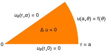
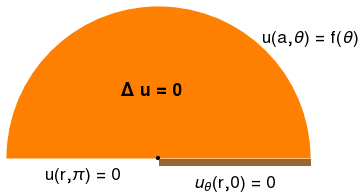
For instance, if we consider the Neumann boundary conditions on the two sides of the wedge,

\[ \begin{split} \frac{1}{r}\, \frac{\partial u}{\partial \theta} = 0 \qquad\mbox{when} \quad \theta = \alpha , \quad r> 0, \\ \frac{1}{r}\, \frac{\partial u}{\partial \theta} = f(r) \qquad\mbox{when} \quad \theta = 0 , \quad r> 0, \end{split} \]
where f is a specified function. Evidently, the solution of the problem, u, is not unique because we can always add c0 + c1 log r, where c0 and c1 are arbitrary constants.

Example: Consider Laplace's equation in a corner:

\[ \begin{split} u_{rr} + \frac{1}{r}\,u_r + \frac{1}{r^2}\, u_{\theta\theta} =0 , \qquad 0 < r < a, \quad 0 < \theta < \alpha , \\ u(r,0) =0 , \quad u(r, \alpha ) =0 , \qquad u(a, \theta ) = f(\theta ) , \\ u(r, \theta ) \ \mbox{ is bounded as }\ r \to 0 \qquad ({\bf wedge\ condition}). \end{split} \]
w = Graphics[{Orange, Disk[{0, 0}, 1, {0, 35 Degree}]}];
text1 = Graphics[ Text[Style["\[CapitalDelta] u = 0", FontSize -> 16], {0.6, 0.2}]];
text2 = Graphics[Text[Style["u = 0", FontSize -> 16], {0.4, 0.4}]]; text3 = Graphics[Text[Style["u = 0", FontSize -> 16], {0.6, -0.05}]]; text4 = Graphics[ Text[Style["u(a,\[Theta]) = f(\[Theta])", FontSize -> 16], {1.18, 0.35}]]; txt0 = Graphics[Text[Style["0", FontSize -> 16], {-0.03, 0.0}]]; txtr = Graphics[Text[Style["r = a", FontSize -> 16], {1.1, 0.0}]]; Show[w, text1, text2, text3, text4, txt0, txtr]
To solve the given boundary value problem, we apply separation of variables. So we seek partial nontrivial (not identically zero) solutions of the auxiliary problem
\[ \begin{split} u_{rr} + \frac{1}{r}\,u_r + \frac{1}{r^2}\, u_{\theta\theta} =0 , \qquad 0 < r < a, \quad 0 < \theta < \alpha , \\ u(r,0) =0 , \quad u(r, \alpha ) =0 , \\ u(r, \theta ) \ \mbox{ is bounded as }\ r \to 0 \qquad ({\bf wedge\ condition}), \end{split} \]
and represented as a product: u(r,θ) = R(r) ⋅ Θ(&theta). Substitution of this product into the Laplace equation yields
\[ r^2 \frac{R'' + \frac{1}{r}\,R'}{R} = - \frac{\Theta'' (\theta )}{\Theta (\theta )} = \lambda^2 , \]
where we denote by λ² the constant of separation. From the above equations, we derive two differential equations containing a parameter λ:
\[ \begin{split} r^2 R'' (r) + r\, R' (r) - \lambda^2 R =0 , \\ \Theta'' (\theta ) + \lambda^2 \Theta (\theta ) =0 , \qquad \Theta (\theta ) = \Theta (\theta + 2 \pi ) . \end{split} \]
The latter is the Sturm--Liouville problem that is not hard to solve:
\[ \Theta_n (\theta ) = \sin \left( \frac{n\pi\theta}{\alpha} \right) \qquad \mbox{for} \quad \lambda_n = \frac{n\pi}{\alpha} , \quad n=1,2,\ldots . \]
Note that λ = 0 is not an eigenvalue because the corresponding eigenfunction Θ0 = a+ bθ must be identically zero to satisfy the homogeneous boundary condition.

Therefore, we get a discrete sequence of positive eigenvalues

\[ \lambda_n = \frac{n\pi}{\alpha} , \quad n=1,2,\ldots , \]
that we will use to solve the Euler differential equation for R(r). If we choose R(r) to be a power function R(r) = rk, we get
\[ R(r) = r^k , \quad r\, R' (r) = k\, r^k , \quad r^2 R'' (r) = k(k-1)\,r^k . \]
So we obtain an algebraic equation for k:
\[ k(k-1) + k - n^2 =0 \qquad \Longrightarrow \qquad k = \pm n. \]
Hence, the general solution for the Euler equation \( r^2 R'' + r\, R' - n^2 R =0 \) becomes
\[ R_n (r) = a_n r^n + b_n r^{-n} , \qquad n=1,2,3,\ldots . \]
Since this function must be bounded at the origin (wedge condition), we are forced to set bn = 0. Adding all nontrivial solution, we obtain
\[ u(r,\theta ) = \sum_{n\ge 1} R_n (t)\, \Theta_n (\theta ) = \sum_{n\ge 1} a_n r^{n\pi /\alpha} \, \sin \left( \frac{n\pi \theta}{\alpha} \right) . \]
To satisfy the boundary condition for r = a, we have to determine the values of coefficients an from the equation
\[ u(a, \theta ) = f(\theta ) = \sum_{n\ge 1} a_n a^{n\pi /\alpha} \, \sin \left( \frac{n\pi \theta}{\alpha} \right) , \]
which is actually the Fourier sine series. Therefore,
\[ a_n = a^{-n\pi/\alpha} \,\frac{2}{\alpha} \int_0^{\alpha} f(\theta )\, \sin \left( \frac{n\pi \theta}{\alpha} \right) {\text d}\theta , \qquad n=1,2,\ldots . \]

Example: Consider the Dirichlet problem for Laplace's equation in a corner:

\[ \begin{split} u_{rr} + \frac{1}{r}\,u_r + \frac{1}{r^2}\, u_{\theta\theta} =0 , \qquad 0 < r < a, \quad 0 < \theta < \alpha , \\ u(r,0) =u_0 , \quad u(r, \alpha ) = u_{\alpha} , \qquad u(a, \theta ) = f(\theta ) , \\ u(r, \theta ) \ \mbox{ is bounded as }\ r \to 0 \qquad ({\bf wedge\ condition}), \end{split} \]
where u0 and uα are given numbers.
w = Graphics[{Orange, Disk[{0, 0}, 1, {0, 35 Degree}]}];
text1 = Graphics[ Text[Style["\[CapitalDelta] u = 0", FontSize -> 16], {0.6, 0.2}]];
text2 = Graphics[ Text[Style[ "u(r,\[Alpha]) = \!\(\*SubscriptBox[\(u\), \(\[Alpha]\)]\)", FontSize -> 16], {0.3, 0.4}]]; text3 = Graphics[ Text[Style["u(r,0) = \!\(\*SubscriptBox[\(u\), \(0\)]\)0", FontSize -> 16], {0.6, -0.05}]]; text4 = Graphics[ Text[Style["u(a,\[Theta]) = f(\[Theta])", FontSize -> 16], {1.18, 0.35}]]; txt0 = Graphics[Text[Style["0", FontSize -> 16], {-0.03, 0.0}]]; txtr = Graphics[Text[Style["r = a", FontSize -> 16], {1.1, 0.0}]]; Show[w, text1, text2, text3, text4, txt0, txtr]
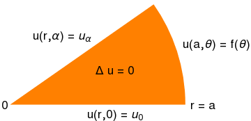
We reduce the given boundary value problem to the problem considered in the previous example with homogeneous boundary conditions by representing the unknown function u(r,θ) as a sum of two functions:
\[ u(r, \theta ) = w(r, \theta ) + v(r, \theta ) , \qquad\mbox{where} \quad w(r, \theta ) = \left( u_{\alpha} - u_0 \right) \frac{\theta}{\alpha} + u_0 . \]
Actually, instead of w can be used any function that satisfies the prescribed boundary conditions: \( w(r,0) = u_0 \) and \( w(r,\alpha ) = u_{\alpha} . \) Then for function v(r,θ) we get the following boundary value problem
\[ \begin{split} v_{rr} + \frac{1}{r}\,v_r + \frac{1}{r^2}\, v_{\theta\theta} =0 , \qquad 0 < r < a, \quad 0 < \theta < \alpha , \\ v(r,0) =0 , \quad v(r, \alpha ) =0 , \qquad v(a, \theta ) = f(\theta ) - w(a,\theta ), \\ v(r, \theta ) \ \mbox{ is bounded as }\ r \to 0 \qquad (\mbox{\bf wedge condition}). \end{split} \]
This is essentially the same problem that was solved in the previous example. ■

Example: .

Consider the Laplace equation subject to mixed boundary conditions:
\[ \begin{split} u_{rr} + \frac{1}{r}\,u_r + \frac{1}{r^2}\, u_{\theta\theta} =0 , \qquad 0 < r < a, \quad 0 < \theta < \alpha , \\ u_{\theta} (r,0) = 0 , \quad u_{\theta} (r, \alpha ) = 0 , \qquad u(a, \theta ) = f(\theta ) , \\ u(r, \theta ) \ \mbox{ is bounded as }\ r \to 0 \qquad ({\bf wedge\ condition}). \end{split} \]
w = Graphics[{Orange, Disk[{0, 0}, 1, {0, 35 Degree}]}];
text1 = Graphics[ Text[Style["\[CapitalDelta] u = 0", FontSize -> 16], {0.6, 0.15}]];
text2 = Graphics[ Text[Style[ "\!\(\*SubscriptBox[\(u\), \(\[Theta]\)]\)(r,\[Alpha]) = 0", FontSize -> 16], {0.3, 0.4}]];
text3 = Graphics[ Text[Style["\!\(\*SubscriptBox[\(u\), \(\[Theta]\)]\)(r,0) = 0", FontSize -> 16], {0.6, -0.05}]];
text4 = Graphics[ Text[Style["u(a,\[Theta]) = f(\[Theta])", FontSize -> 16], {1.18, 0.35}]]; txt0 = Graphics[Text[Style["0", FontSize -> 16], {-0.03, 0.0}]]; txtr = Graphics[Text[Style["r = a", FontSize -> 16], {1.1, 0.0}]]; Show[w, text1, text2, text3, text4, txt0, txtr]

Example: Consider the boundary value problem for the Laplace equation in circular domain:

\[ \begin{split} u_{rr} + \frac{1}{r}\,u_r + \frac{1}{r^2}\, u_{\theta\theta} =0 , \qquad a < r < b, \quad \alpha < \theta < \beta , \\ u_{\theta} (r,0) = 0 , \quad u_{\theta} (r, \alpha ) = 0 , \qquad u(a, \theta ) = g(\theta ) , \quad u(b, \theta ) = f(\theta ) . \end{split} \]
w = RegionPlot[ 1/2 <= x^2 + y^2 <= 2 && 0 < x && x < y , {x, 0, 2.1}, {y, 0, 2}, Frame -> False, PlotStyle -> LightOrange];
text1 = Graphics[ Text[Style["\[CapitalDelta] u = 0", FontSize -> 16, FontWeight -> "Bold"], {0.4, 1.0}]];
text2 = Graphics[ Text[Style["u(r,\[Beta]) = 0", FontSize -> 16], {-0.3, 0.74}]];
text3 = Graphics[ Text[Style["u(r,\[Alpha]) = 0", FontSize -> 16], {1.0, 0.75}]];
text4 = Graphics[ Text[Style["u(b,\[Theta]) = f(\[Theta])", FontSize -> 16], {0.8, 1.4}]];
text5 = Graphics[ Text[Style["u(a,\[Theta]) = g(\[Theta])", FontSize -> 16], {0.3, 0.45}]];
Show[w, text1, text2, text3, text4, text5]

Example: Consider the boundary value problem for Laplace's equation

\[ \begin{split} u_{rr} + \frac{1}{r}\,u_r + \frac{1}{r^2}\, u_{\theta\theta} =0 , \qquad 0 < r < a, \quad 0 < \theta < \pi , \\ u_{\theta} (r,0) = 0 , \quad u (r, \pi ) = 0 , \qquad u(a, \theta ) = f(\theta ) , \end{split} \]
w = Graphics[{Orange, Disk[{0, 0}, 1, {0, Pi}]}];
text1 = Graphics[ Text[Style["\[CapitalDelta] u = 0", FontSize -> 16, FontWeight -> "Bold"], {-0.05, 0.45}]];
text2 = Graphics[ Text[Style["\!\(\*SubscriptBox[\(u\), \(\[Theta]\)]\)(r,0) = 0", FontSize -> 16], {0.5, -0.15}]];
text3 = Graphics[ Text[Style["u(r,\[Pi]) = 0", FontSize -> 16], {-0.5, -0.1}]];
text4 = Graphics[ Text[Style["u(a,\[Theta]) = f(\[Theta])", FontSize -> 16], {1.0, 0.8}]];
p = Graphics[{PointSize[Medium], Point[{0, 0}]}];
rec = Graphics[{Brown, Rectangle[{1, -0.05}, {0, 0}]}];
Show[w, text1, text2, text3, text4, p, rec]

Substituting the assumed form u(r,θ) = R(r) ⋅ Θ(&theta) into Laplace's equation, and separating variables, we obtain two differential equations

\[ \begin{split} r^2 R;; (r) + r\,R' (r) - \lambda^2 R(r) =0 , \\ \Theta'' (\theta ) + \lambda^2 \Theta (\theta ) =0 . \end{split} \]
Adding the boundary conditions at θ = 0 and θ = π, we get the Sturm--Liouville problem:
\[ \Theta'' (\theta ) + \lambda^2 \Theta (\theta ) =0 , \qquad \Theta' (0) =0, \quad \Theta (\pi ) =0. \]
So we derive the eigenvalues and corresponding eigenfunctions:
\[ \Theta_n (\theta ) = \cos \left( \frac{\theta \left( 1 + 2n \right)}{2} \right) , \qquad \lambda_n = \frac{\left( 1 + 2n \right)}{2} , \qquad n=0,1,2,\ldots . \]
Note that λ = 0 is not an eigenvalue. Then the solution to the given boundary value problem is the sum of all partial nontrivial solutions
\[ u (r,\theta ) = \sum_{n\ge 0} c_n \,r^(n+1/2) \,\cos \left( \frac{\theta \left( 1 + 2n \right)}{2} \right) . \]
To satisfy the boundary condition at r = a, we have to choose coefficients cn so that
\[ u (a,\theta ) = f(\theta ) = \sum_{n\ge 1} c_n \,a^{n+1/2} \,\cos \left( \frac{\theta \left( 1 + 2n \right)}{2} \right) . \]
Since this is just Fourier series over orthogonal set of eigenfunctions, we determine its coefficients as
\[ c_n = a^{-n-1/2} \,\frac{2}{\pi} \int_0^{\pi} f(\theta )\,\cos \left( \frac{\theta \left( 1 + 2n \right)}{2} \right) {\text d}\theta , \quad n=0,1,2, \ldots . \]

Example: Consider the boundary value problem for Laplace's equation

\[ \begin{split} u_{rr} + \frac{1}{r}\,u_r + \frac{1}{r^2}\, u_{\theta\theta} =0 , \qquad 0 < r < a, \quad 0 < \theta < 2\pi , \\ u_{\theta} (r,0+0) = u_0 , \quad u (r, 2\pi -0 ) = u_1 , \qquad u(a, \theta ) = f(\theta ) , \end{split} \]

w = Graphics[{Orange, Disk[{0, 0}, 1, {0.01, 2*Pi - 0.01}]}];
p = Graphics[{PointSize[Medium], Point[{0, 0}]}];
text1 = Graphics[ Text[Style["\[CapitalDelta] u = 0", FontSize -> 16, FontWeight -> "Bold"], {-0.05, 0.45}]];
text2 = Graphics[ Text[Style["u(r,0+0) = \!\(\*SubscriptBox[\(u\), \(0\)]\)(r)", FontSize -> 16], {0.5, 0.1}]];
text3 = Graphics[ Text[Style["u(r,2\[Pi]-0) = \!\(\*SubscriptBox[\(u\), \(1\)]\)(r)", FontSize -> 16], {0.5, -0.1}]];
text4 = Graphics[ Text[Style["u(a,\[Theta]) = f(\[Theta])", FontSize -> 16], {1.0, 0.8}]];
Show[w, text1, text2, text3, text4, p, rec]

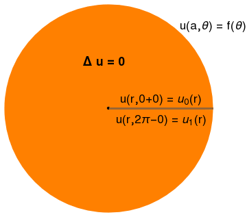
If the boundary conditions on the crack are the same, u0 = u1, the solution can be obtained from our first two examples by taking the limit \( \lim_{\alpha \to 2\pi} u(r, \theta ) . \) When they are not the same, the problem becomes very hard to solve. ■

Laplace equation in a corner


  1. Peirce, A., Circular domains, 2018.


Return to Mathematica page

Return to the main page (APMA0340)
Return to the Part 1 Matrix Algebra
Return to the Part 2 Linear Systems of Ordinary Differential Equations
Return to the Part 3 Non-linear Systems of Ordinary Differential Equations
Return to the Part 4 Numerical Methods
Return to the Part 5 Fourier Series
Return to the Part 6 Partial Differential Equations
Return to the Part 7 Special Functions