Preface
This section studies some first order nonlinear ordinary differential equations describing the time evolution (or “motion”) of those hamiltonian systems provided with a first integral linking implicitly both variables to a motion constant. An application has been performed on the Lotka--Volterra predator-prey system, turning to a strongly nonlinear differential equation in the phase variables.
Return to computing page for the second course APMA0340
Return to Mathematica tutorial for the first course APMA0330
Return to Mathematica tutorial for the second course APMA0340
Return to the main page for the first course APMA0330
Return to the main page for the second course APMA0340
Return to Part I of the course APMA0340
Introduction to Linear Algebra with Mathematica
Glossary
Double pendulum
 |
 |
 |
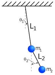
A double pendulum consists of one pendulum attached to another. Double pendula are an example of a simple physical system which can exhibit chaotic behavior with a strong sensitivity to initial conditions. Several variants of the double pendulum may be considered. The two limbs may be of equal or unequal lengths and masses; they may be simple pendulums/pendula or compound pendulums (also called complex pendulums) and the motion may be in three dimensions or restricted to the vertical plane.
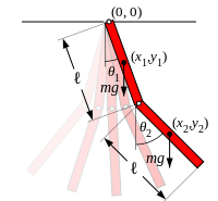
Consider a double bob pendulum with masses m1 and m2, attached by rigid massless wires of lengths \( \ell_1 \) and \( \ell_2 . \) Further, let the angles the two wires make with the vertical be denoted \( \theta_1 \) and \( \theta_2 , \) as illustrated at the left. Let the origin of the Cartesian coordinate system is taken to be at the point of suspension of the first pendulum, with vertical axis pointed up. Finally, let gravity be given by g. Then the positions of the bobs are given by
sol = First[ NDSolve[{2*phi1''[t] + phi2''[t]*Cos[phi1[t] - phi2[t]] +
phi2'[t]^(2)*Sin[phi1[t] - phi2[t]] + 2*9.81*Sin[phi1[t]] == 0,
phi2''[t] + phi1''[t]*Cos[phi1[t] - phi2[t]] - phi1'[t]^(2)*Sin[phi1[t] - phi2[t]] + 9.81*Sin[phi2[t]] == 0,
phi1[0] == Pi/2, phi2[0] == Pi, phi1'[0] == 0,
phi2'[0] == 0}, {phi1[t], phi2[t]}, {t, 0, 10}]];
x1[t_] := Evaluate[Sin[phi1[t]] /. sol]
y1[t_] := Evaluate[-Cos[phi1[t]] /. sol]
x2[t_] := Evaluate[Sin[phi1[t]] + Sin[phi2[t]] /. sol]
y2[t_] := Evaluate[-(Cos[phi1[t]] + Cos[phi2[t]]) /. sol]
frames = Table[ Graphics[{Gray, Thick,
Line[{{0, 0}, {x1[t], y1[t]}, {x2[t], y2[t]}}], Darker[Blue],
Disk[{0, 0}, .1], Darker[Red], Disk[{x1[t], y1[t]}, .1],
Disk[{x2[t], y2[t]}, .1]}, PlotRange -> {{-2.5, 2.5}, {-2.5, 2.5}}], {t, 0, 10, .1}];
ListAnimate[frames]
The equations of motion can also be written in the Hamiltonian formalism. Computing the generalized momenta gives
Double pendulum animation:
Manipulate[
 Module[{eqns, \[Theta]1, \[Theta]2, sol, pos1, pos2, t, pq, path},
  eqns = {(m1 + m2) l1 \[Theta]1''[t] +
      m2 l2 \[Theta]2''[t] Cos[\[Theta]1[t] - \[Theta]2[t]] +
      m2 l2 \[Theta]2'[t]^2 Sin[\[Theta]1[t] - \[Theta]2[t]] +
      g (m1 + m2) Sin[\[Theta]1[t]] == 0,
    m2 l2 \[Theta]2''[t] +
      m2 l1 \[Theta]1''[t] Cos[\[Theta]1[t] - \[Theta]2[t]] -
      m2 l1 \[Theta]1'[t]^2 Sin[\[Theta]1[t] - \[Theta]2[t]] +
      m2 g Sin[\[Theta]2[t]] == 0, \[Theta]1[0] ==
     init1, \[Theta]2[0] == init2, \[Theta]1'[0] ==
     initprime1, \[Theta]2'[0] == initprime2};
  sol = NDSolve[eqns, {\[Theta]1, \[Theta]2}, {t, 0, p},
    MaxSteps -> Infinity, PrecisionGoal -> 4];
  pq = sol[[1, 1, 2, 1, 1, 2]];
  pos1[t_] := {l1 Sin[\[Theta]1[t]], -l1 Cos[\[Theta]1[t]]};
  pos2[t_] := {(l1 Sin[\[Theta]1[t]] +
      l2 Sin[\[Theta]2[t]]), (-l1 Cos[\[Theta]1[t]] -
      l2 Cos[\[Theta]2[t]])};
  path = ParametricPlot[
    Evaluate[pos2[t] /. sol[[1]]], {t, p - p/5, p},
    ColorFunction -> (Directive[Lighter[Blue, .3], Opacity[0.66 #3]] &)
    (*makes it faster,
    but introduces blue points--a bug in ParametricPlot*),
    MaxRecursion -> ControlActive[2, 4]];
  Column[{Graphics[{GrayLevel[.4, .6], Circle[{0, 0}, l1],
      Darker[Blue, .2], path[[1]],
      Line[Evaluate[{pos1[pq], pos2[pq]} /. sol]],
      Disk[First@Evaluate[pos2[pq] /. sol], .2], Darker[Green, .2],
      Line[{{0, 0}, First@Evaluate[pos1[pq] /. sol]}],
      Disk[First@Evaluate[pos1[pq] /. sol], .2]},
     ImageSize -> {320, 300},
     PlotRange -> {{-(l1 + l2) - .5, (l1 + l2) + .5}, {(l1 +
           l2) + .5, -(l1 + l2) - .5}}],
    g1[t_?NumberQ] =
     Switch[plottype,
       heights, -l1 Cos[\[Theta]1[t]], \[Theta]\[Theta], \[Theta]1[
        t], \[Theta]\[Theta]prime1, \[Theta]1[
        t], \[Theta]\[Theta]prime2, \[Theta]2[t], _, 1] /. sol[[1]];
    g2[t_?NumberQ] =
     Switch[plottype,
       heights, (-l1 Cos[\[Theta]1[t]] -
         l2 Cos[\[Theta]2[t]]), \[Theta]\[Theta], \[Theta]2[
        t], \[Theta]\[Theta]prime1, \[Theta]1'[
        t], \[Theta]\[Theta]prime2, \[Theta]2'[t], _, 1] /. sol[[1]];
    Switch[plottype, heights,
     Plot[{g1[t], g2[t]}, {t, 0, p},
      MaxRecursion -> ControlActive[3, 4], PlotStyle -> {Green, Blue},
       Axes -> False,
      PlotLabel -> Style["pendulum positions", "Label"],
      PlotRange -> {{pq - 10, pq}, Automatic},
      ImageSize -> {320, 100},
      AspectRatio -> 32/100.], \[Theta]\[Theta],
     ParametricPlot[{g1[t], g2[t]}, {t, 0, p},
      MaxRecursion -> ControlActive[3, 4], Axes -> False,
      PlotLabel ->
       Row[{Subscript[\[Theta], 1], " vs. ", Subscript[\[Theta], 2]}],
       PlotRange -> {{-Pi, Pi}, Automatic}, ImageSize -> {320, 100},
      ColorFunction -> (Blend[{Blue, Green}, #1] &),
      AspectRatio -> 32/100.], \[Theta]\[Theta]prime1,
     ParametricPlot[{g1[t], g2[t]}, {t, 0, p},
      MaxRecursion -> ControlActive[3, 4], Axes -> False,
      PlotLabel ->
       Row[{Subscript[\[Theta], 1], " vs. ",
         Subscript[OverDot[\[Theta]], 1]}],
      PlotRange -> {{-Pi, Pi}, Automatic}, ImageSize -> {320, 100},
      AspectRatio -> 32/100.,
      PlotStyle -> Darker[Green, .2]], \[Theta]\[Theta]prime2,
     ParametricPlot[{g1[t], g2[t]}, {t, 0, p},
      MaxRecursion -> ControlActive[3, 4], Axes -> False,
      PlotLabel ->
       Row[{Subscript[\[Theta], 2], " vs. ",
         Subscript[OverDot[\[Theta]], 2]}],
      PlotRange -> {{-Pi, Pi}, Automatic}, ImageSize -> {320, 100},
      AspectRatio -> 32/100., PlotStyle -> Darker[Blue, .2]], _,
     Graphics[{White, Point[{0, 0}]}]]}, Dividers -> None]],
 Style["constants", "SubSection", Bold], {{m1, 3, "green mass"}, 1,
  10, ImageSize -> Tiny, ContinuousAction -> False,
  Appearance -> "Labeled"}, {{m2, 1, "blue mass"}, 1, 10,
  ImageSize -> Tiny, Appearance -> "Labeled",
  ContinuousAction -> False}, {{l1, 1, "green length"}, 1, 3,
  ImageSize -> Tiny, ContinuousAction -> False,
  Appearance -> "Labeled"}, {{l2, 1.5, "blue length"}, 1, 3,
  ImageSize -> Tiny, Appearance -> "Labeled",
  ContinuousAction -> False}, {{g, 9.8, "gravity"}, 5, 15,
  ImageSize -> Tiny, Appearance -> "Labeled",
  ContinuousAction -> False}, Delimiter,
 Style["initial conditions", "SubSection",
  Bold], {{init1, Pi/2, "green angle"}, -Pi, Pi,
  Appearance -> "Labeled",
  ImageSize -> Tiny}, {{init2, 0, "blue angle"}, -Pi, Pi,
  Appearance -> "Labeled",
  ImageSize -> Tiny}, {{initprime1, 0, "green velocity"}, -10, 10,
  ImageSize -> Tiny,
  Appearance -> "Labeled"}, {{initprime2, -3, "blue velocity"}, -10,
  10, ImageSize -> Tiny,
  Appearance -> "Labeled"}, Delimiter, {{p, 12, "time"}, 0.00001, 100,
   ImageSize -> Tiny}, {{plottype, heights,
   "plot"}, {heights -> "positions", \[Theta]\[Theta] ->
    "\!\(\*SubscriptBox[\(\[Theta]\), \(1\)]\) vs. \
\!\(\*SubscriptBox[\(\[Theta]\), \(2\)]\)", \[Theta]\[Theta]prime1 ->
    "\!\(\*SubscriptBox[\(\[Theta]\), \(1\)]\) vs. \
\!\(\*SubscriptBox[OverscriptBox[\(\[Theta]\), \(.\)], \(1\)]\)", \
\[Theta]\[Theta]prime2 ->
    "\!\(\*SubscriptBox[\(\[Theta]\), \(2\)]\) vs. \
\!\(\*SubscriptBox[OverscriptBox[\(\[Theta]\), \(.\)], \(2\)]\)"},
  ControlType -> PopupMenu}, AutorunSequencing -> {{10, 10}, 11},
 TrackedSymbols :> {m1, m2, l1, l2, g, init1, init2, initprime1,
   initprime2, plottype, p}]
|
|
Using the NDSolve function on Mathematica, it is possible to evaluate each angle as time moves forward from 0 to 0.15 seconds. 101 frames are then produced by evaluating the position of the shoulder, wrists, and clubhead with respect to time, with each frame being 3.6 milliseconds apart. A table is then formulated to include the graphics of each line and disc. Two dotted lines and a second blue disk are arbitrarily plotted to visually represent the right shoulder and arm. With this animation, it is possible to evaluate the dynamics of the golf swing: the upward accelerating left shoulder, the torque-driven left arm, and the free wrists that release the golf club through the bottom of the downswing. A side-by-side comparison is made with an actual golf swing, which features similar parameters and torques to the pendulum model.
After analyzing the animation, data is drawn from the Lagrangian differential equation to give a more detailed look at both speeds and horizontal angles in the swing. First, the speeds of both the clubhead and the hands are calculated using the magnitude of vertical and horizontal velocities. Here, it is seen that the clubhead travels at a maximum of 57.87 meters per second, or roughly 130 miles per hour. However, this is assuming no wrist torque which is only accurate before contact. In order to find the time of contact, it is assumed that the ball is hit while the clubhead is travelling perfectly level to the ground (zero degrees to the horizontal). This is an average "angle of attack" for a professional golfer. Using the second plot, which displays this attack angle with respect to time (with horizontal and vertical velocities overlaid for reference), it is found that impact occurs at t = 0.247142 seconds. At this time, the clubhead speed is determined to be 49.95 meters per second, roughly 112 miles per hour. The average clubhead speed value on the PGA Tour is approximately 114 mph, proving an accurate result.
By incorporating Lagrangian and non-linear differential equations, the dynamics of the golf swing can be better understood and represented for positive benefit. For example, it is seen here that the vertical acceleration of the left shoulder combined with a fairly free wrist-club torque produces a faster clubhead speed, with relatively slow hand speed. It is also seen that with the loose wrist model, clubhead speed continues to increase after the angle of attack is perfectly horizontal, explaining why some of the best drivers of the golf ball tend to make contact while the club is travelling slightly upwards, by 2 or 3 degrees. Eventually, stiffness in the wrist and ball-flight inefficiencies limit this advantage. With more dynamic and mathematical analysis, there is potential to locate areas of the golf swing that would produce a more efficient golf swing, leading to faster swing speeds and longer drives.
In this model of the golf swing, the arms and golf club are simplified into a double-pendulum system (seen below)
Defining Variables
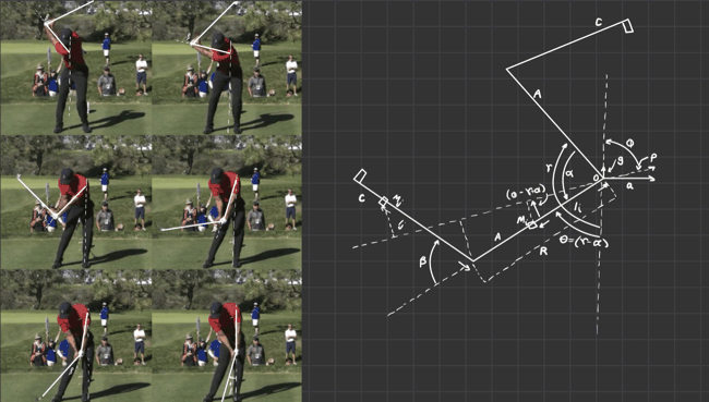
CL - club,
γ - angle between arms and vertical direction,
α - descendant angle of arms,
β - descendant angle of club,
θ - (γ − α)
R - length of arms A,
Ii - distance from (mi) to origin,
Ij - distance from (mj) to origin,
SA = first moment of arms about origin,
MC = mass of the club,
S - first moment of club about wrist,
\( J = \sum_i m_i \ell_i^2 , \) - second moment of rod A about axis,
\( I = \sum_j m_j \ell_j^2 , \) - second moment of rod CL about axis,
g = upward acceleration of gravity,
a = horizontal acceleration of golfer.
Modeling the swing
Generalized torque
Mathematica codes
α = Pi - phi1[t]
β = phi2[t] - phi1[t]
\( \dot{\alpha} = \) phi1'[t]
\( \dot{\beta} = \) phi2'[t] − phi1'[t]
\( \ddot{\alpha} = \) phi1''[t]
\( \ddot{\beta} = \) phi2''[t] − phi1''[t]
eqn2 = Ic (phi2''[t] - phi1''[t]) - (Ic + R*S*Cos[(phi2[t] - phi1[t])]) (phi1''[t]) + (phi1'[t])^2*R*S* Sin[(phi2[t] - phi1[t])] + S (g*Sin[phi1[t] + (phi2[t] - phi1[t])] - a*Cos[phi1[t] + phi2[t] - phi1[t]]) == Qb;
sol = First[ NDSolve[{(J + Ic + MC*R^2 + 2 R*S*Cos[(phi2[t] - phi1[t])]) (phi1''[ t]) - (Ic + R*S*Cos[(phi2[t] - phi1[t])]) (phi2''[t] - phi1''[t]) + (((phi2'[t] - phi1'[t]))^2 - 2 (phi1'[t])*(phi2'[t] - phi1'[t])) R*S* Sin[(phi2[t] - phi1[t])] - S (g*Sin[phi1[t] + (phi2[t] - phi1[t])] - a*Cos[phi1[t] + (phi2[t] - phi1[t])]) - (SA + MC*R) (g*Sin[phi1[t]] - a*Cos[phi1[t]]) == Qa, Ic (phi2''[t] - phi1''[t]) - (Ic + R*S*Cos[(phi2[t] - phi1[t])]) (phi1''[t]) + (phi1'[t])^2*R* S*Sin[(phi2[t] - phi1[t])] + S (g*Sin[phi1[t] + (phi2[t] - phi1[t])] - a*Cos[phi1[t] + phi2[t] - phi1[t]]) == Qb, phi1[0] == 5.5 Pi/4, phi2[0] == 5 Pi/8 , phi1'[0] == 0, phi2'[0] == 0}, {phi1[t], phi2[t]}, {t, 0, 0.0036, .36}]];;
x1[t_] := Evaluate[R*(Sin[phi1[t]] /. sol)];
y1[t_] := Evaluate[R*(-Cos[phi1[t]] /. sol) + a*t];
x2[t_] := Evaluate[R*Sin[phi1[t]] + CL*Sin[phi2[t]] /. sol];
y2[t_] := Evaluate[(-(R*Cos[phi1[t]] + CL*Cos[phi2[t]]) /. sol) + a*t];
frames = Table[ Graphics[{Gray, Thick, Line[{{0, a*t}, {x1[t], y1[t]}, {x2[t], y2[t]}}], {Dotted, Line[{{-.3 + t, (t - .2)^2}, {0, a*t}}]}, {Dotted, Line[{{-.3 + t, (t - .2)^2}, {x1[t], y1[t]}}]}, Darker[Green], Line[{{-2.5, -1.6}, {2.5, -1.6}}], Darker[Blue], Disk[{0, a*t}, .1], Disk[{-.3 + t, (t - .2)^2}, .1], Darker[White], Disk[{x1[t], y1[t]}, .08], Darker[Black], Disk[{x2[t], y2[t]}, .1]}, PlotRange -> {{-2.5, 2}, {-2.5, 2}}], {t, 0, .36, .0036}];
p1 = Import[ "/Users/ray.gresalfi/Desktop/GolfSwingz123.mov", {"Frames", Range[1, 101]}];
xy = Transpose[{frames, p1}] // Partition[#, 1] &;
ani = ListPlot[#] & /@ xy;
ListAnimate[xy, ImageSize -> Full, AnimationRunning -> False]
clubheadspeed = ((x2'[t])^2 + (y2'[t]^2))^.5; handspeed = ((x1'[t])^2 + (y1'[t]^2))^.5; Plot[{clubheadspeed, handspeed}, {t, 0, .36}, AxesLabel -> {"time", "Speed"}, PlotLabels -> {"Clubhead Speed", "Hand Speed"}]
FindMaximum[{clubheadspeed, 0 <= t <= .247142}, t] anglehoriz = N[ArcTan[x2'[t], y2'[t]] /Degree];
Plot[{x2'[t], y2'[t], anglehoriz}, {t, .2, .3}, PlotStyle -> {Dotted, Dotted, Thick}, AxesLabel -> {"time", "angle(d)/velocity(m/s)"}, PlotLabels -> {"Horizontal Velocity", "Vertical Velocity", "Attack Angle"}]
FindRoot[anglehoriz, {t, .2}]
- Jorgensen, Theodore P. The Physics of Golf. 2 ed., New York, Springer-Verlag, 1994.
- Pickering, and Vickers. On the Double Pendulum Model of the Golf Swing, Sports Engineering, vol. 2, 1999, pp. 161-172. Wiley Online Library.
Return to Mathematica page
Return to the main page (APMA0340)
Return to the Part 1 Matrix Algebra
Return to the Part 2 Linear Systems of Ordinary Differential Equations
Return to the Part 3 Non-linear Systems of Ordinary Differential Equations
Return to the Part 4 Numerical Methods
Return to the Part 5 Fourier Series
Return to the Part 6 Partial Differential Equations
Return to the Part 7 Special Functions