Return to computing page for the second course APMA0340
Return to Mathematica tutorial for the first course APMA0330
Return to Mathematica tutorial for the second course APMA0340
Return to the main page for the first course APMA0330
Return to the main page for the second course APMA0340
Return to Part III of the course APMA0340
Introduction to Linear Algebra with Mathematica
Glossary
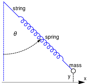
Spring Pendulum
sols = NDSolve[{r''[t] + (k/m)*(r[t] - l0) - r[t]*(theta'[t])^2 - g*Cos[theta[t]] == 0, theta''[t] + (2/r[t])*r'[t]*theta'[t] + (g/r[t])*Sin[theta[t]] == 0, r[0] == 3, r'[0] == -0.5, theta[0] == 0.5, theta'[0] == 0.1}, {r, theta}, {t, 0, 100}];
ParametricPlot[{r[t], r'[t]} /. sols, {t, 0, 50}] ParametricPlot[{theta[t], theta'[t]} /. sols, {t, 0, 50}]
Spring Pendulum
|
coil = ParametricPlot[{(t + 0.5*Sin[6*t])/Sqrt[2] +
0.5*Cos[6 t]/Sqrt[2], -(t + 0.5*Sin[6*t])/Sqrt[2] +
0.5*Cos[6*t]/Sqrt[2]}, {t, -0.27, 4*Pi + 0.26}, PlotStyle -> {Thick, Blue}] line1 = Graphics[{Thick, Blue, Line[{{-0.5, 0.5}, {-4, 4}}]}] line2 = Graphics[{Thick, Blue, Line[{{9.4, -9.4}, {11.4, -11.4}}]}] line3 = Graphics[{Thick, Blue, Dashed, Line[{{-4, -14}, {-4, 4}}]}] circle = Graphics[{Thick, Circle[{11.8, -11.8}, 0.5]}] circle2 = Graphics[{Thick, Dashed, Circle[{-4, 4}, 12, {-Pi/2, -Pi/4}]}] arrow = Graphics[{Arrowheads[0.05], Arrow[{{4.46 - 0.3, -4.46 - 0.3}, {4.46, -4.46}}]}] text = Graphics[Style[Text["\[Theta]", {-1.4, -3.3}], FontSize -> 22]] mass = Graphics[Style[Text["mass", {12.3, -10.5}], FontSize -> 20]] spring = Graphics[Style[Text["spring", {7, -4}], FontSize -> 20]] string = Graphics[Style[Text["string", {-0.5, 2.5}], FontSize -> 20]] xarrow = Graphics[{Arrowheads[0.08], Arrow[{{-4.4, -14.4}, {14.5, -14.4}}]}] x = Graphics[Style[Text["x", {14.5, -13.5}], FontSize -> 20]] line4 = Graphics[{Thick, Dashed, Line[{{11.8, -12.5}, {11.8, -14.3}}]}] y = Graphics[Style[Text["y", {10.9, -13.0}], FontSize -> 20]] Show[line1, line2, coil, circle, line3, circle2, arrow, text, mass, spring, string, xarrow, x, line4, y] |
|
| Figure 1: Spring pendulum m > 0. | Mathematica code |
History of spring pendulum:
Planar oscillations of elastic (spring) pendulum was first considered by Vitt, A. (Aleksandr Adolʹfovich) and Gorelik, G. (Gabriel Simonovich) in 1933. Its translation from the Russian in English by Lisa Shields with an introduction by Peter Lynch is available on the web.
The problem investigated by Vitt & Gorelik has only two degrees of freedom, namely the vertical and one of the horizontal dimensions. According to Gabriel Gorelik, the study was motivated by the Russian physicist L. I. Mandelshtam, who suggested this research topic as a worthy analogue of the recurrence phenomenon in the infrared spectrum of CO2, which is known today as Fermi resonance. It could serve as an analogue of less accessible systems such as the frequency doubling of laser light in a nonlinear crystal. Of particular interest is the case where the frequency of the vertical motion is exactly or nearly twice the frequency of the horizontal. Under those circumstances the vertical oscillations become parametrically unstable, and any small initial deviation of the bob from the vertical line through the spring support results in exponentially increasing horizontal (or pendulum) oscillation. The growth of the latter stops eventually, as most of the energy of the original vertical oscillations is converted into energy of pendulum motion. The process is now reversed as the centrifugal force, with two cycles of oscillation in the pendulum period, acts as a forcing or excitation term to the vertical harmonic oscillations. This phenomenon is a called parametric resonance of the coupled system, which manifests itself as an energy transfer from one component to the other and vice versa. The speed and amplitude of the energy transfer depend essentially on the initial conditions.The elastic pendulum has been analyzed previously, either as a mechanical problem, or in conjunction with other parametric phenomena, such as wave-wave coupling in plasma physics and non-linear optics, and also in the problem of the coupling of vertical and radial oscillations of particles in cyclic accelerators. The applied mathematician, the popularizer of mathematics, research meteorologist, academic, and Irish Times columnist Peter Lynch (Dublin) initialized a research on wide class of systems modeled by an integrable approximation to the 3 degrees of freedom elastic pendulum with 1:1:2 resonance, or the swing-spring. He explained the phenomenon of the splitting of the spectral lines in the CO2 molecule (Raman scattering). This simple system under study possesses a rich and varied range of dynamical behavior. It has many analogues in other areas. For example, electrical systems with two degrees of freedom can be treated in similar ways, e.g., two oscillating circuits coupled by a transformer with an iron core.
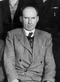
Gabriel Gorelik was born into a Jewish family in Paris in 1909. He later studied theoretical physics under Mandelstam in Lomonosov Moscow State University, and then worked under A.A. Andronov, where he was later bullied in 1952 for his "ideological mistakes," as were many others at the time. Gorelik was tragically killed by a train in 1956. Gorelik's father, Simon, sacrificed his own life to save Moscow from a pneumonia plague outbreak in 1939 by diagnosing the disease, and then locking himself and the infected people inside the building while trying to save the life of the microbiologist Berlin, so that only twelve people died from the plague, including Simon Gorelik. Aleksandr Adolfovich Vitt also suffered a tragic fate. Vitt was born in Russia in 1902 to ethnic German parents, and he also studied under Mandelstam then later Andronov. Vitt was then persecuted during the Great Purge in 1938 and was sentenced to 5 years of labor camps where he died soon after 1938.
 |
 |
 |
 |
||
|---|---|---|---|---|---|
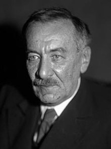
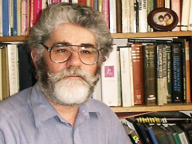
| Leonid Mandelshtam. | Peter Lynch. | Gabriel Gorelik. | Alexander Vitt. |
Leonid Isaakovich Mandelstam, or Mandelshtam (1879--1944) was a Soviet physicist of Belarusian-Jewish background. Leonid Mandelstam was born in Mogilev, Russian Empire (now Belarus). He studied at the Novorossiya University in Odessa, but was expelled in 1899 due to political activities, and continued his studies at the University of Strasbourg. He remained in Strasbourg until 1914, and returned with the beginning of World War I. He was awarded the Stalin Prize in 1942. Mandelstam died in Moscow, USSR (now Russia). He was a co-discoverer of inelastic combinatorial scattering of light used now in Raman spectroscopy. In 1918, Mandelstam theoretically predicted the fine structure splitting in Rayleigh scattering due to light scattering on thermal acoustic waves. Beginning from 1926, L.I. Mandelstam and G.S. Landsberg initiated experimental studies on vibrational scattering of light in crystals at the Moscow State University. As a result of this research, Landsberg and Mandelstam discovered the effect of the combinatorial scattering of light on 21 February 1928. They presented this fundamental discovery for the first time at a colloquium on 27 April 1928. They published brief reports about this discovery (experimental results with theoretical explanation) in Russian and in German, then they published a comprehensive paper in Zeitschrift fur Physik.
Current interest in the swinging spring arises from the rich variety of its solutions. The swinging and springing oscillations act as analogues of the Rossby and gravity waves in the atmosphere and may provide the basis for a paradigm of the most important interannual variation in the ocean-atmosphere climate system. For very small amplitudes, the motion is regular. As the amplitude is increased, the regular motion breaks down into a chaotic regime that occupies more and more of phase space as the energy grows. However, for very large energies, a regular and predictable regime is re-established (see Núñez-Yépez etal). This can easily be understood: for very high energies, the system rotates rapidly around the point of suspension and is no longer vibratory.
The elastic pendulum problem became well known to the public after publication in 1947 of the famous book "Introduction to Non-Linear Mechanics" by Nicolas Minorsky (1885--1970). Nikolai Fyodorovich Minorsky was a Russian American control theory mathematician, engineer, and applied scientist. He is best known for his theoretical analysis and first proposed application of PID controllers in the automatic steering systems for U.S. Navy ships. He was educated at the Nikolaev Maritime Academy in St. Petersburg (Russia), and at the University of Nancy (France). For a year in 1917 to 1918 he was the adjunct Naval Attache at the Russian Embassy to France in Paris. In the midst of the Russian civil war Minorsky emigrated to the United States in June 1918.
From 1924–1934 Nicolas Minorsky was a Professor of Electronics and Applied Physics at the University of Pennsylvania. He received his PhD in physics from Penn in 1929. Minorsky worked on roll stabilization of ships for the Navy from 1934 to 1940, designing in 1938 an activated-tank stabilization system into a 5-ton model ship. His work was used for stabilizing of aircraft carriers during the landing of airplanes.
Our exposition of elastic pendulum follows the Minorsky's book. Let us consider a massless spring of rest length \( \ell_0 \) hung with a bob of mass m on its lower end; also let r be its length under load, k the spring constant, and g the acceleration of gravity. We assume that the pendulum is constrained to move in a fixed vertical plane, with the origin at the pivot when Cartesian coordinates or polar coordinates are employed. Obviously the system possesses two degrees of freedom, namely, the angle θ of the pendulum and the elongation r of the spring.
★Let \( \ell = \ell_0 + \frac{mg}{k} \) be the length of the spring at equilibrium when the bob is attached because \( k \left( \ell - \ell_0 \right) = mg , \) where k is the spring constant in Hooke's law. The deviation from the loaded equilibrium is described in rectangular coordinates as
In order to derive the system of differential equations that model the spring pendulum oscillations, we calculate its kinetic energy
-
Vitt, A. (Aleksandr Adolʹfovich) and Gorelik, G. (Gabriel Simonovich), Oscillations of an Elastic Pendulum as an Example of the Oscillations of Two
Parametrically Coupled Linear Systems,
Journal of Technical Physics, 1933, vol. 3, pp. 294–307.
Its translation from the Russian in English by Lisa Shields with an introduction by Peter Lynch is available on the web:
http://copac.jisc.ac.uk/id/15694518?style=html
http://catalogue.nli.ie/Record/vtls000058645 - T. R. Kane and M. E. Kahn, On a Class of Two-Degree-of-Freedom Oscillations, Journal of Applied Mechanics, ASME, Volume 35, Issue 3, pp. 547--552; doi:10.1115/1.3601249
- E., Breitenberger and R.D. Mueller, The elastic pendulum: A nonlinear paradigm, Journal of Mathematical Physics, 22, 1196 (1981); https://doi.org/10.1063/1.525030
- Yahli Narkis, On the stability of a spring-pendulum, Zeitschrift für angewandte Mathematik und Physik, March 1977, Volume 28, Issue 2, pp 343--348
- H.N. Núñez-Yépez, A.L. Salas-Brito, C.A. Vargas, and L. Vicente, 1990: Onset of chaos in an extensible pendulum, Physics Letters A, A145, Issues 2-3, pp. 101--105; https://doi.org/10.1016/0375-9601(90)90199-X
- Tsel'man, P.Kh., On pumping transfer of energy between nonlinearly coupled oscillators in third-order resonance, PMM, 34, No. 5, 1970, pp. 957--962.
3D Elastic Pendulum

The spring-mass oscillator is generally presumed to be one of the simplest and most basic physical systems. In the previous section, we considered massless spring with attached bob of mass m. Because a real spring has a finite distributed mass, we consider the bob that is suspended on a homogeneous elastic spring of mass ms with the elasticity constant k. The three dimensional spring pendulum was considered by P. Pokorny in 2008. Our exposition of this problem follows closely Pavel Pokorny's article
Denoting the rectangular coordinates of the bob by X, Y, and Z, and assuming the spring is stretched homogeneously, the kinetic energy of the system consisting of the spring with the bob becomes
-
Витт А. А., Горелик Г. С. Колебания упругого маятника как пример двух параметрически связанных линейных систем, Журнал технической физики, т. 3 (2-3) 294--306 1933.
Vitt, A. (Aleksandr Adolʹfovich) and Gorelik, G. (Gabriel Simonovich), Oscillations of an Elastic Pendulum as an Example of the Oscillations of Two
Parametrically Coupled Linear Systems,
Journal of Technical Physics, 1933, vol. 3, pp. 294–307.
Its translation from the Russian in English by Lisa Shields with an introduction by Peter Lynch is available on the web:
http://copac.jisc.ac.uk/id/15694518?style=html
http://catalogue.nli.ie/Record/vtls000058645 -
P. Pokorny, Stability condition for vertical oscillation of 3-dim heavy spring elastic pendulum,
Regular and Chaotic Dynamics,
June 2008, Volume 13, Issue 3, pp 155--165.
https://link.springer.com/article/10.1134/S1560354708030027
http://old.vscht.cz/mat/Pavel.Pokorny/rcd/RCD155-color.pdf - Pendulum Wikipedia
- Pendulum Physics
- Lumen Physics: Pendulum
- Predicting the Future – An Intro to Models Described by Time Dependent Differential Equations by Christian J Howard.
- Salas, A.H. and Castillo, J.E., Exact Solution to Duffing Equation and the Pendulum Equation, Applied Mathematical Sciences, Vol. 8, 2014, no. 176, 8781 - 8789; http://dx.doi.org/10.12988/ams.2014.44243
- M. G. Olsson, Why does a mass on a spring sometimes misbehave?, American Journal of Physics, 44, Issue 12, 1211 (1976); https://doi.org/10.1119/1.10265
- Casey, J., Geometrical derivation of Lagrange’s equations for a system of particles, American Journal of Physics, 62(9) 836–847 (1994). https://doi.org/10.1119/1.17470
- Corey Zammit, Nirantha Balagopal, Zijun Li, Shenghao Xia, and Qisong Xiao, The dynamic of the elastic pendulum, Arizona.
- Qisong Xiao; Shenghao Xia; Corey Zammit; Nirantha Balagopal; Zijun Li, Dynamics of the Elastic Pendulum, Arizona.
- C. Madigan, The Spring Pendulum, MapleSoft.
- K. Craig, Spring-pendulum dynamic system, NYU, 2001.
Wilberforce Pendulum
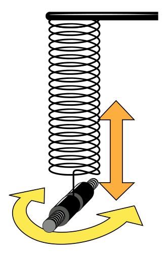
A Wilberforce pendulum, invented by British physicist Lionel Robert Wilberforce (1861--1944) around 1896, consists of a mass suspended by a long helical spring and free to turn on its vertical axis, twisting the spring. It is an example of a coupled mechanical oscillator, often used as a demonstration in physics education. The mass can both bob up and down on the spring, and rotate back and forth about its vertical axis with torsional vibrations. When correctly adjusted and set in motion, it exhibits a curious motion in which periods of purely rotational oscillation gradually alternate with periods of purely up and down oscillation. The energy stored in the device shifts slowly back and forth between the translational 'up and down' oscillation mode and the torsional 'clockwise and counterclockwise' oscillation mode, until the motion eventually dies away.
Let us consider a massless spiral spring with a longitudinal spring constant k and a torsional constant δ, on which a mass m is attached having a moment of inertia about its vertical axis, I. Assuming a linear coupling of the form εzθ/2, where the two coordinates are z and θ, and z = θ = 0 is the equilibrium point, we can write the Lagrangean for the system as
The Euler--Lagrange equations of motion are