Preface
This section is devoted to an important class of nonlinear system of equations---gradient systems. The reason why gradient systems are grouped together is that for such systems there is a natural candidate for a Lyapunov function.
Return to computing page for the first course APMA0330
Return to computing page for the second course APMA0340
Return to Mathematica tutorial for the first course APMA0330
Return to Mathematica tutorial for the second course APMA0340
Return to the main page for the first course APMA0330
Return to the main page for the second course APMA0340
Return to Part III of the course APMA0340
Introduction to Linear Algebra
Glossary
Gradient Systems
Today, more than three centuries after Isaac Newton wrote down his treatise on the theory of fluxions, and after the rise of the calculus of variations, it has turned out that a large number of evolution models may be expressed in the mathematical language of ordinary and partial differential equations. A system of the form
Suppose that the function G(x) has an isolated local minimum/maximum value at the point x*. Then this point will be a critical point of the given system of differential equations. Its orbits follow the path of steepest descent/increase of G depending on the sign of k.
Let \( U \subset \mathbb{R}^n \) be an open set and let \( G\,:U \to \mathbb{R}^n \) be a continuous function. A function \( E\,: U \to \mathbb{R} \) is called an energy function for the first order vector differential equation
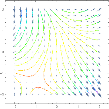
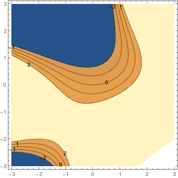
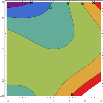
The gradient (denoted by nabla: ∇) is an operator that associates a vector field to a scalar field. Both scalar and vector fields may be naturally represented in Mathematica as pure functions. However, there is no built-in Mathematica function that computes the gradient vector field (however, there is a special symbol \[ EmptyDownTriangle ] for nabla). The command Grad gives the gradient of the input function. In Mathematica, the main command to plot gradient fields is VectorPlot. Here is an example how to use it.
f[x_, y_] := x^2 + y^2 *x - 3*y
VectorPlot[Gradf, {x, xmin, xmax}, {y, ymin, ymax},
StreamPoints -> Coarse, StreamColorFunction -> Hue]]
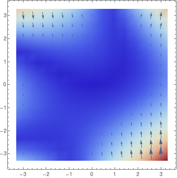
VectorDensityPlot[{y, x^2 + y^2*x - 3*y}, {x, -3, 3}, {y, -3, 3}, ColorFunction -> "ThermometerColors"][
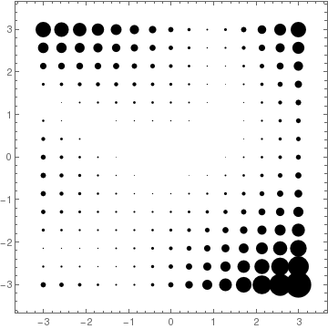
VectorPlot[{y, x^2 + y^2*x - 3*y}, {x, -3, 3}, {y, -3, 3}, VectorStyle -> {Black, "Disk"}]
 |
 |
 |
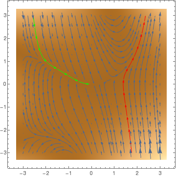
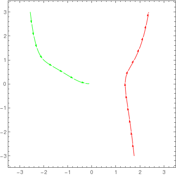
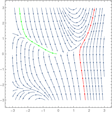
StreamPlot[{y, x^2 + y^2*x - 3*y}, {x, -3, 3}, {y, -3, 3}, StreamPoints -> {{{{-2, 1}, Green}, {{1.5, -1}, Red}, Automatic}}]
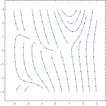
StreamPlot[{y, x^2 + y^2*x - 3*y}, {x, -3, 3}, {y, -3, 3}, StreamPoints -> Coarse]
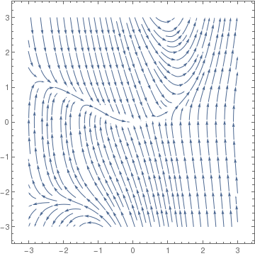
StreamPlot[{y, x^2 + y^2*x - 3*y}, {x, -3, 3}, {y, -3, 3}, StreamPoints -> Fine]
 |
 |
 |
 |
 |
 |
Module[
{
img,
cont,
densityOptions,
contourOptions,
frameOptions,
gradField,
field,
fieldL,
plotRangeRule,
rangeCoords
},
densityOptions = Join[
FilterRules[{opts},
FilterRules[Options[DensityPlot],
Except[{Prolog, Epilog, FrameTicks, PlotLabel, ImagePadding, GridLines,
Mesh, AspectRatio, PlotRangePadding, Frame, Axes}]]],
{PlotRangePadding -> None, Frame -> None, Axes -> None, AspectRatio -> Automatic}
];
contourOptions = Join[
FilterRules[{opts},
FilterRules[Options[ContourPlot],
Except[{Prolog, Epilog, FrameTicks, PlotLabel, Background,
ContourShading, PlotRangePadding, Frame, Axes, ExclusionsStyle}]]],
{PlotRangePadding -> None, Frame -> None, Axes -> None,
ContourShading -> False}
];
gradField = ComplexExpand[{D[f, rx[[1]]], D[f, ry[[1]]]}];
fieldL =
DensityPlot[Norm[gradField], rx, ry,
Evaluate@Apply[Sequence, densityOptions]];
field=First@Cases[{fieldL},Graphics[__],\[Infinity]];
img = Rasterize[field, "Image"];
plotRangeRule = FilterRules[Quiet@AbsoluteOptions[field], PlotRange];
cont = If[
MemberQ[{0, None}, (Contours /. FilterRules[{opts}, Contours])],
{},
ContourPlot[f, rx, ry, Evaluate@Apply[Sequence, contourOptions]]
];
frameOptions = Join[
FilterRules[{opts},
FilterRules[Options[Graphics],
Except[{PlotRangeClipping, PlotRange}]]],
{plotRangeRule, Frame -> True, PlotRangeClipping -> True}
];
rangeCoords = Transpose[PlotRange /. plotRangeRule];
If[Head[fieldL]===Legended,Legended[#,fieldL[[2]]],#]&@
Apply[Show[
Graphics[
{
Inset[
Show[SetAlphaChannel[img,
"ShadingOpacity" /. {opts} /. {"ShadingOpacity" -> 1}],
AspectRatio -> Full], rangeCoords[[1]], {0, 0},
rangeCoords[[2]] - rangeCoords[[1]]]
}],
cont,
StreamPlot[gradField, rx, ry,
Evaluate@FilterRules[{opts}, StreamStyle],
Evaluate@FilterRules[{opts}, StreamColorFunction],
Evaluate@FilterRules[{opts}, StreamColorFunctionScaling],
Evaluate@FilterRules[{opts}, StreamPoints],
Evaluate@FilterRules[{opts}, StreamScale]],
##
] &, frameOptions]
]
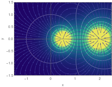
2) - (y^2 + (x - 1/2)^2)^(-1/2)/2, {x, -1.5, 3.5}, {y, -1.5, 1.5},
PlotPoints -> 50, ColorFunction -> "BlueGreenYellow", Contours -> 16,
ContourStyle -> White, Frame -> True, FrameLabel -> {"x", "y"},
ClippingStyle -> Automatic, StreamStyle -> Orange, ImageSize -> 500,
GridLinesStyle -> Directive[Thick, Black], "ShadingOpacity" -> .8,
Axes -> {True, False}, AxesStyle -> Directive[Thickness[.03], Black],
Method -> {"AxesInFront" -> False}]
How to recognize a gradient system
Equilibria and their stability
- If the eigenvalues of the Hessian are all strictly positive, then the critical point is asymptotically stable.
- If the Hessian has a negative real eigenvalue, then the equilibrium is unstable.
Example: This seems to have Let
|
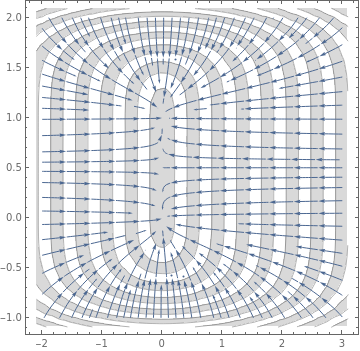
StreamPlot[{-6*x, -2*y*(y - 1)*(2*y - 1)}, {x, -2, 3}, {y, -1, 2},
Mesh -> 18, MeshShading -> {LightGray, None},
PlotTheme -> "Detailed"]
|
|
| Figure 1: Gradient system. | Mathematica code |
■
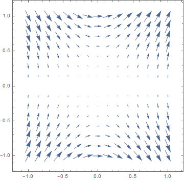
D[f[x, y], {{x, y}}]
VectorPlot[%, {x, -1, 1}, {y, -1, 1}]
- Calle Ysern, B., Asymptotically stable equilibria of gradient systems, American Mathematical Monthly, 2019, Vol. 126, No. 10, pp. 936--939.
- Hirsch, M.W., Smale, S., and Devaney, R.L., Differential Equations, Dynamical Systems, and an Introduction to Chaos, 2003, Second edition, Academic Press.
Return to Mathematica page
Return to the main page (APMA0340)
Return to the Part 1 Matrix Algebra
Return to the Part 2 Linear Systems of Ordinary Differential Equations
Return to the Part 3 Non-linear Systems of Ordinary Differential Equations
Return to the Part 4 Numerical Methods
Return to the Part 5 Fourier Series
Return to the Part 6 Partial Differential Equations
Return to the Part 7 Special Functions