Preface


This tutorial was made solely for the purpose of education and it was designed for students taking Applied Math 0340. It is primarily for students who have some experience using Mathematica. If you have never used Mathematica before and would like to learn more of the basics for this computer algebra system, it is strongly recommended looking at the APMA 0330 tutorial. As a friendly reminder, don't forget to clear variables in use and/or the kernel. The Mathematica commands in this tutorial are all written in bold black font, while Mathematica output is in normal font.

Finally, you can copy and paste all commands into your Mathematica notebook, change the parameters, and run them because the tutorial is under the terms of the GNU General Public License (GPL). You, as the user, are free to use the scripts for your needs to learn the Mathematica program, and have the right to distribute and refer to this tutorial, as long as this tutorial is accredited appropriately. The tutorial accompanies the textbook Applied Differential Equations. The Primary Course by Vladimir Dobrushkin, CRC Press, 2015; http://www.crcpress.com/product/isbn/9781439851043

Return to computing page for the first course APMA0330
Return to computing page for the second course APMA0340
Return to Mathematica tutorial for the first course APMA0330
Return to Mathematica tutorial for the second course APMA0340
Return to the main page for the first course APMA0330
Return to the main page for the second course APMA0340
Introduction to Linear Algebra with Mathematica

Introduction: Tubing


Consider a curve in three-dimensional space defined parametrically by

\[ x = f(t), \quad y = g(t), \quad z=h(t). \]
We are interested in finding an equation of the surface with a circular cross section of radius a that surrounds this curve, which is a tube that follows the shape of the curve. A point P on the desired surface can be reached by adding two vectors: r(t) that connects the origin with a point on the curve and a vector a(u) that connects that point to a point on the surface. If P denotes the position vector of point P, then
\[ {\bf P}(t,u) \equiv \left\langle X(t,u), Y(t,u), Z(t,u) \right\rangle = {\bf r}(t) + {\bf a} (u) . \]
The first vector r(t) has components \( \left\langle f(t), g(t), h(t) \right\rangle , \) corresponding to the parametrization of the curve, and the second vector has components
\[ {\bf a}(u) = \left\langle a\,\cos (u)\,\cos\varphi , a\,\cos (u)\,\sin\varphi , a\,\sin (u) \right\rangle , \]
where u is the angle that a(u) makes with cylindrical unit vector \( \hat{\bf e}_{\rho} \) and ϕ is the angle that \( \hat{\bf e}_{\rho} \) makes with the positive ordinate. We need to express coordinates of P as a function of two paramters. Expressing trigonometric functions as functions of t, we get
\[ \cos \varphi = \frac{x}{\rho} = \frac{f(t)}{\sqrt{f^2 (t) + g^2 (t)}} , \qquad \sin \varphi = \frac{y}{\rho} = \frac{g(t)}{\sqrt{f^2 (t) + g^2 (t)}} . \]
Then we derive
\[ \begin{split} X(t,u) &= f(t) + a\,\cos u\,\cos \varphi = f(t) \left( 1 + \frac{a\,\cos u}{\sqrt{f^2 (t) + g^2 (t)}} \right) , \\ Y(t,u) &= g(t) + a\,\cos u\,\sin \varphi = g(t) \left( 1 + \frac{a\,\cos u}{\sqrt{f^2 (t) + g^2 (t)}} \right) , \\ Z(t,u) &= h(t) + a\,\sin u . \end{split} \]
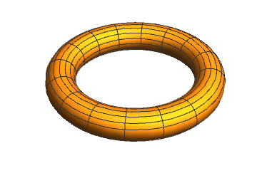
Finally, we plot some equations with Mathematica. We start with torus:
f[t_] := 5*Cos[t]; g[t_] := 5*Sin[t]; h[t_] := 0;
X[t_, u_, a_] := f[t] (1 + a*Cos[u]/Sqrt[f[t]^2 + g[t]^2])
Y[t_, u_, a_] := g[t] (1 + a*Cos[u]/Sqrt[f[t]^2 + g[t]^2])
Z[t_, u_, a_] := h[t] + a*Sin[u]
ParametricPlot3D[{X[t, u, 1], Y[t, u, 1], Z[t, u, 1]}, {t, 0, 2*Pi}, {u, 0, 2*Pi}, Axes -> False, Boxed -> False]
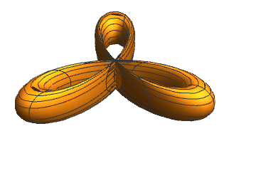
Next, we produce the tubing of a clover leaf.
Clear[f, g]
f[t_] := 5*Cos[t]*Cos[3*t]; g[t_] := 5*Sin[t]*Cos[3*t];
ParametricPlot3D[{X[t, u, 1], Y[t, u, 1], Z[t, u, 1]}, {t, 0, 2*Pi}, {u, 0, 2*Pi}, Axes -> False, Boxed -> False, PlotPoints -> 30]
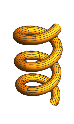
The third plot is a helicl tube.
Clear[f, g, h]
f[t_] := 4*Cos[t]; g[t_] := 4*Sin[t]; h[t_] := t;
ParametricPlot3D[{X[t, u, 1], Y[t, u, 1], Z[t, u, 1]}, {t, 0, 6*Pi}, {u, 0, 6*Pi}, Axes -> False, Boxed -> False, PlotPoints -> 30]
By replacing the functions f, g, and h with any other triplet, one can produce a variety of tubes. However, as the figure with clover tube shows, the circular cross sectons are not really circular. A true circular cross section should describe a circle perpendicular to the curve.

To make the circular cross section perpendicular to the curve, we have to choose a(u) to be of constant length and perpendicular to the curve at the point of contact. This means that a(u) is to be perpendicular to an element of length dr of the curve. Since

\[ {\text d}{\bf r} = \left\langle {\text d}f , {\text d}g , {\text d}h \right\rangle = \left\langle f' (t) , g' (t) , h' (t) \right\rangle {\text d}t, \]
a(u) must be perpendicular to \( {\bf r}' (t) \equiv \left\langle f' (t) , g' (t) , h' (t) \right\rangle . \) Letting a(u) have components s, v, and w, we have
\[ {\bf r}' (t) \cdot {\bf a} (u) = 0 = \left\langle f' (t) , g' (t) , h' (t) \right\rangle \cdot \left\langle s , v , w \right\rangle . \]
This equation can be rewritten in Mathematica as
r[t_] := {f[t],g[t], h[t]}; rp = {s,v,w} ;
r'[t] . rp == 0
where we have used rp for a(u). We need to define an angle uon the circular sross section to measure the direction of a(u). For this, we need a fiducial axis relative to which we measure the angle. This axis must lie on the plane of the circle. A vector that defines such an axis could be taken to be \( \left\langle h' (t) , 0 , -f' (t) \right\rangle . \) Therefore, we get the second equation

horV := {h'[t], 0, -f'[t]} ;
Cos[u] == horV . rp / (a*Sqrt[h'[t]^2 + f'[t]^2])
where a is the length of the vector rp:
rp.rp == a^2 ;
We ask Mathematica to solve the above three equations.
Solve[{{f'[t],g'[t], h'[t]}. {s,v,w} ==0, Cos[u] == (s*h'[t] - w*f'[t])/(a*Sqrt[h'[t]^2 + f'[t]^2]), s^2 + h^2 + g^2 == a^2}, {s,v,w}]
The result is a list of solutions with very long expressions. We simplify the output:
FullSimplify[%]
The solution contains two values for each component of rp. We want to choose the first one for each, say
s/.%
Then we extract the first choice typing in either
Part[%,1]
or
First[%]
This yields
\[ ah' \left( \frac{\cos u}{\sqrt{f'^2 + h'^2}} + \frac{a\, \sin^2 u \,f' g'^2}{\sqrt{a^2 \sin^2 u \, f'^2 g'^2 \left( f'^2 + h'^2 \right) \left( f'^2 + g'^2 + h'^2 \right)}} \right) . \]
To extract the powers out of radical we apply PowerExpand to the expression.
S[t_, u_, a_] := PowerExpand[%]
This is what we called s before, but now we have explicit expressions
\[ S(t,u,a) = \frac{ah' \,\cos u}{\sqrt{f'^2 + h'^2}} + \frac{a\, \sin u \,f' g'}{\sqrt{\left( f'^2 + h'^2 \right) \left( f'^2 + g'^2 + h'^2 \right)}} . \]
Similarly, we can define
\[ V(t,u,a) = - \frac{a\, \sin u \,\sqrt{f'^2 + h'^2}}{\sqrt{f'^2 + g'^2 + h'^2}} \]
for v and
\[ W(t,u,a) = -\frac{af' \,\cos u}{\sqrt{f'^2 + h'^2}} + \frac{a\, \sin u \,f' g'}{\sqrt{\left( f'^2 + h'^2 \right) \left( f'^2 + g'^2 + h'^2 \right)}} \]
for w.


Return to Mathematica page

Return to the main page (APMA0340)
Return to the Part 1 Matrix Algebra
Return to the Part 2 Linear Systems of Ordinary Differential Equations
Return to the Part 3 Non-linear Systems of Ordinary Differential Equations
Return to the Part 4 Numerical Methods
Return to the Part 5 Fourier Series
Return to the Part 6 Partial Differential Equations
Return to the Part 7 Special Functions