Return to computing page for the first course APMA0330
Return to computing page for the second course APMA0340
Return to Mathematica tutorial for the first course APMA0330
Return to Mathematica tutorial for the second course APMA0340
Return to the main page for the first course APMA0330
Return to the main page for the second course APMA0340
Return to Part II of the course APMA0340
Introduction to Linear Algebra with Mathematica

Preface


This section is devoted to second order linear differential equations.

Second order systems of equations

Differential equations of arbitrary order with constant coefficients can be solved in straightforward matter by converting them into system of first order ODEs. However, they also can be solved directly, as we demonstrate shortly upon considering second order equations.

Consider a second order vector differential equation

\begin{equation} \label{EqSecond.1} \ddot{\bf x} + {\bf A} \, {\bf x} = {\bf 0} , \end{equation}
subject to the initial conditions
\begin{equation} \label{EqSecond.2} {\bf x} (0) = {\bf d} \qquad\mbox{and} \qquad \dot{\bf x} (0) = {\bf v} , \end{equation}
where A is a n × n square matrix, d and v are initial displace ments and velocities, and x(t) is a column-vector of n unknown functions to be determined. Its solution
\begin{equation} \label{EqSecond.3} {\bf x}(t) = {\bf \Psi}(t)\,{\bf d} + {\bf \Phi}(t)\, {\bf v}, \end{equation}
is expressed through two fundamental matrices
\begin{equation} \label{EqSecond.4} {\bf \Psi}(t) = \cos \left( \sqrt{\bf A}\, t\right) \qquad\mbox{and} \qquad {\bf \Phi}(t) = \dfrac{\sin \left( \sqrt{\bf A} \,t \right)}{\sqrt{\bf A}}, \end{equation}
and d and v are initial displacements and velocities, that is, \( {\bf x}(0) = {\bf d} \) and \( \dot{\bf x}(0) = {\bf v} .\) These two fundamental matrices are solutions of the same matrix differential equation of the second order \( \ddot{\bf P}(t) + {\bf A}\,{\bf P} = {\bf 0}, \) but distinct initial conditions:
\begin{equation} \label{EqSecond.5} \ddot{\bf \Psi} + {\bf A} \, {\bf \Psi} = {\bf 0} , \quad {\bf \Psi}(0) = {\bf I}, \quad \dot{\bf \Psi}(0) = {\bf 0}, \qquad \mbox{and} \qquad \ddot{\bf \Phi} + {\bf A} \, {\bf \Phi} = {\bf 0} , \quad {\bf \Phi}(0) = {\bf 0}, \quad \dot{\bf \Phi}(0) = {\bf I}. \end{equation}
It can verified by direct substitution that the solution \( {\bf x}(t) = {\bf \Psi}(t)\,{\bf d} + {\bf \Phi}(t)\, {\bf v} \) of the vector second order differential equation \( \ddot{\bf x} (t) + {\bf A} \, {\bf x} = {\bf 0} \) satisfies the initial conditions:
\[ {\bf x}(0) = {\bf d} \qquad\mbox{and} \qquad \dot{\bf x}(0) = {\bf v} . \]
The above formula can be obtained using the Laplace transform. Indeed, application of the Laplace transformation, we reduce the given initial value problem to the algebraic equation:
\[ \lambda^2 {\bf x}^L - \dot{\bf x} (0) - \lambda \,{\bf x}(0) + {\bf A}\,{\bf x}^L = {\bf 0} , \]
where
\[ {\bf x}^L = {\cal L} [{\bf x} ] = \int_0^{\infty} {\bf x}(t)\,e^{\lambda t} \, {\text d}t \]
is the Laplace transform of the unknown vector function x(t). Solving the above linear algebraic equation, we obtain
\[ {\bf x}^L = \left( \lambda^2 {\bf I} + {\bf A} \right)^{-1} \left[ \dot{\bf x} (0) + \lambda \,{\bf x}(0) \right] \qquad\Longrightarrow \qquad {\bf x}^L = \frac{\bf d}{\lambda^2 {\bf I} + {\bf A}} + \frac{\lambda {\bf v}}{\lambda^2 {\bf I} + {\bf A}} . \]
Using well known formulas for the inverse Laplace transformations:
\[ {\cal L}^{-1} \left[ \frac{1}{\lambda^2 {\bf I} + {\bf A}} \right] = \frac{\sin \left( \sqrt{\bf A}\,t \right)}{\sqrt{\bf A}} , \qquad {\cal L}^{-1} \left[ \frac{\lambda}{\lambda^2 {\bf I} + {\bf A}} \right] = \cos \left( \sqrt{\bf A}\,t \right) , \]
we arrive at the general solution formula.

This problem can also be solved by converting the given second order vector differential equation to the system of first order differential equations

\[ \dot{\bf y} = {\bf B}\,{\bf y} , \]
where \( {\bf y}(t) = \langle {\bf x}, \dot{\bf x} \rangle \) is 2n column vector of displacements and velocities, and B is a corresponding \( 2n \times 2n \) matrix:
\[ {\bf B} = \begin{bmatrix} {\bf 0} & {\bf I} \\ - {\bf A} & {\bf 0} \end{bmatrix} , \]
where I is the identity n×n matrix. The characteristic polynomial for matrix B becomes
\[ \det \left( \lambda {\bf I} - {\bf B} \right) = \det \left( \lambda^4 {\bf I} - {\bf A} \right) . \]
However, this approach is not optimal and requires more efforts, as it will be shown by examples.    ■
Example 1: Consider the initial value problem for the second order vector differential equation
\[ \ddot{\bf x} + {\bf A}\,{\bf x} = {\bf 0} , \qquad {\bf x}(0) = \begin{bmatrix} 1 \\ 2 \end{bmatrix} , \quad \dot{\bf x}(0) = \begin{bmatrix} -1 \\ -1 \end{bmatrix} , \]
where
\[ {\bf A} = \left[ \begin{array}{cc} \phantom{-}16& -9 \\ -12 & 13 \end{array} \right] . \]
First, we find its eigenvalues and eigenvectors:
A = {{16, -9}, {-12, 13}}
Eigensystem[A]
{{25, 4}, {{-1, 1}, {3, 4}}}
So the matrix A has two positive eigenvalues 4 and 25 (such matrices are called positive). ■


Second Order Homogeneous Equations


Homogeneous second order systems of differential equation with constant coefficients in normal form can be written as
\begin{equation} \label{EqSecond.6} \ddot{\bf x} + {\bf B} \, \dot{\bf x} + {\bf A} \, {\bf x} = {\bf 0} , \qquad {\bf x}(0) = {\bf d} , \quad \dot{\bf x}(0) = {\bf v} . \end{equation}
Here A and B are n × n matrices with constant entries. When initial conditions \eqref{EqSecond.2} are specified, we get the vector initial value problem that can be solved by the Laplace transform.
Example 2: Consider the initial value problem for the second order vector differential equation
\[ \ddot{\bf x} + {\bf B}\,\dot{\bf x} + {\bf A}\,{\bf x} = {\bf 0} , \qquad {\bf x}(0) = \begin{bmatrix} 1 \\ 2 \end{bmatrix} , \quad \dot{\bf x}(0) = \begin{bmatrix} -1 \\ -1 \end{bmatrix} , \]
where
\[ {\bf A} = \left[ \begin{array}{cc} \phantom{-}16& -9 \\ -12 & 13 \end{array} \right] , \qquad {\bf B} = \left[ \begin{array}{cc} \phantom{-}16& -9 \\ -12 & 13 \end{array} \right] \]
First, we find its eigenvalues and eigenvectors:
A = {{16, -9}, {-12, 13}}
Eigensystem[A]
{{25, 4}, {{-1, 1}, {3, 4}}}
So the matrix A has two positive eigenvalues 4 and 25 (such matrices are called positive). ■


Second Order Inhomogeneous Equations


Nonhomogeneous second order systems of differential equation with constant coefficients can be solved in straightforward matter based on the Laplace transform. Indeed, consider the initial value problem:
\[ \ddot{\bf x} + {\bf B} \, \dot{\bf x} + {\bf A} \, {\bf x} = {\bf f}(t) , \qquad {\bf x}(0) = {\bf d} , \quad \dot{\bf x}(0) = {\bf v} . \]
Application of the Laplace transform yields
\[ \lambda^2 {\bf x}^L + \lambda\,{\bf B}\,{\bf x}^L + {\bf A} \, {\bf x}^L = {\bf d} + \lambda {\bf v} + {\bf B}\,{\bf x}^L + {\bf f}^L . \]
Therefore, the Laplace transform of the unknown function x(t) is expressed explicitly:
\[ {\bf x}^L = \frac{{\bf d} + \lambda {\bf v} + {\bf B}}{\lambda^2 {\bf I} + \lambda \,{\bf B} + {\bf A}} + \frac{1}{\lambda^2 {\bf I} + \lambda \,{\bf B} + {\bf A}} \, {\bf f}^L , \]
where \( {\bf f}^L = \int_0^{\infty} {\bf f}(t)\, e^{-\lambda t}\,{\text d}t \) is the Laplace transform of the input function f. This allows us to determine the solution by apllying the inverse Laplace transform:
\[ {\bf x} (t) = {\cal L}^{-1} \left[ \frac{{\bf d} + \lambda {\bf v} + {\bf B}}{\lambda^2 {\bf I} + \lambda \,{\bf B} + {\bf A}} \right] + {\cal L}^{-1} \left[ \frac{1}{\lambda^2 {\bf I} + \lambda \,{\bf B} + {\bf A}} \, {\bf f}^L \right] . \]


(which means that all its eigenvalues are positive)


Example 3:
Example 2:

Consider the second order vector differential equation \( \ddot{\bf x} + {\bf A}\,{\bf x} = {\bf 0} ,\) where

\[ {\bf A} = \left[ \begin{array}{cc}
1& 4 & 16 \\ 18& 20 & 4 \\ -12 & -14 & -7 \end{array} \right] . \]

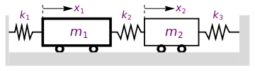
Example 11: When a system with masses connected by springs is in motion, the springs are subject to both elongation and compression. It is clear from experience that there is some force, called the restoring force, which tends to return the attached mass to its equilibrium position. According to Hooke's law, the restoring force has direction opposite to the elongation (or compression) and is proportional to the distance of the mass from its equilibrium position. The corresponding constant of proportionality is called a spring constant.

We consider a situation when two bodies of masses m1 and m2 that are connected to three springs of negligible mass having spring constants k1 k2, and k3, respectively. We denote by x1 and x2 displacement of each body from its equilibrium position.

     
mass1 = Graphics[{Thickness[0.01], Line[{{-12.5, 0.5}, {-2.5, 0.5}, {-2.5, 4.5}, {-12.5, 4.5}, {-12.5, 0.5}}]}, Ticks -> None, Axes -> False];
mass2 = Graphics[{Thickness[0.01], Line[{{2.5, 0.5}, {2.5, 4.5}, {10.5, 4.5}, {10.5, 0.5}, {2.5, 0.5}}]}, Ticks -> None, Axes -> False];
spring1 = Graphics[{Thickness[0.005], Line[{{-12.5, 2.5}, {-14, 2.5}, {-14.4, 1.5}, {-14.8, 3.5}, {-15.2, 1.5}, {-15.6, 3.5}, {-16, 1.5}, {-16.4, 3.5}, {-16.6, 2.5}, {-17.5, 2.5}}]}, Ticks -> None, Axes -> False];
spring2 = Graphics[{Thickness[0.005], Line[{{-2.5, 2.5}, {-1.5, 2.5}, {-1, 1.5}, {-0.5, 3.5}, {0, 1.5}, {0.5, 3.5}, {1, 1.5}, {1.5, 3.5}, {2, 2.5}, {2.5, 2.5}}]}, Ticks -> None, Axes -> False];
spring3 = Graphics[{Thickness[0.005], Line[{{10.5, 2.5}, {11.5, 2.5}, {12, 1.5}, {12.5, 3.5}, {13, 1.5}, {13.5, 3.5}, {14, 1.5}, {14.5, 3.5}, {15, 2.5}, {16.5, 2.5}}]}, Ticks -> None, Axes -> False];
c1 = Graphics[{Thickness[0.01], Circle[{-10, 0}, 0.5]}];
c2 = Graphics[{Thickness[0.01], Circle[{-5, 0}, 0.5]}];
c3 = Graphics[{Thickness[0.01], Circle[{5, 0}, 0.5]}];
c4 = Graphics[{Thickness[0.01], Circle[{8, 0}, 0.5]}];
polygon = Graphics[{LightGray, Polygon[{{-17.5, -0.5}, {16.5, -0.5}, {16.5, -2.5}, {-17.5, -2.5}}]}];
poly1 = Graphics[{LightGray, Polygon[{{-17.5, -2.5}, {-18, -2.5}, {-18, 5}, {-17.5, 5}}]}];;
poly2 = Graphics[{LightGray, Polygon[{{16.5, -2.5}, {18, -2.5}, {18, 5}, {16.5, 5}}]}];
l1 = Graphics[{Dashed, Line[{{-12.5, 4.5}, {-12.5, 6.5}}]}];
l2 = Graphics[{Dashed, Line[{{2.5, 4.5}, {2.5, 6.5}}]}];
a1 = Graphics[Arrow[{{-12.5, 6}, {-8, 6}}]];
a2 = Graphics[Arrow[{{2.5, 6}, {7, 6}}]];
txt1 = Graphics[ Text[Style[Subscript[x, 1], FontSize -> 14, Purple], {-7, 6}]];
txt2 = Graphics[ Text[Style[Subscript[x, 2], FontSize -> 14, Purple], {8, 6}]];
t1 = Graphics[ Text[Style[Subscript[m, 1], FontSize -> 18, Purple], {-7, 2.5}]];
t2 = Graphics[ Text[Style[Subscript[m, 2], FontSize -> 18, Purple], {7, 2.5}]];
k1 = Graphics[ Text[Style[Subscript[k, 1], FontSize -> 14, Purple], {-15, 5}]];
k2 = Graphics[ Text[Style[Subscript[k, 2], FontSize -> 14, Purple], {0, 5}]];
k3 = Graphics[ Text[Style[Subscript[k, 3], FontSize -> 14, Purple], {13.5, 5}]];
Show[mass1, mass2, spring1, spring2, spring3, c1, c2, c3, c4, polygon, poly1, poly2, l1, l2, a1, a2, txt1, txt2,t1,t2,k1,k2,k3]
       Spring-mass system.            Mathematica code

This example can be used to model several mechanical systems because there are many situations when we observe masses connected with each other. For example, a multi-story building can be considered as masses (corresponding to each floor) connecting with springs. You can model an entire set of automobiles with several hundred masses connected to each other by several undred springs and can analyze how each part of the whole car vibrates when you drive this caravan along a bumpy road. Or you can model an entire set of rail cars with several masses, one for each car and one for the locomotive, all connected to each other by several springs and then analyze how each part of the whole train vibrates when the train chugs along climbing the mountain rail. You may think this kind of simple two mass and three spring model is not adequate for complicated models from real life, but in reality the logic and process of modeling is exactly the same. You would just have several dozens of differential equations instead of two or three equations, which is very similar to what you see here.

Let x1 and x2 be displacements of masses m1 and m2, respectively, from their equilibrium positions. So we consider these variables as canonical coordinates. Then the kinetic energy of these two objects will be

\[ \mbox{K} = \frac{1}{2}\,m_1 \dot{x}_1^2 + \frac{1}{2}\,m_2 \dot{x}_2^2 , \]
where \( \dot{x} = {\text d}x/{\text d}t \) is the velocity corresponding to the displacement x. The potential energy is concentrated in three springs and it is equal to the sum of potential energies of each spring. Correspondingly, the potential energy of each spring is proportional to the square of the amount the spring is stretched, so
\[ \Pi = \frac{1}{2}\,k_1 x_1^2 + \frac{1}{2}\,k_2 \left( x_1 - x_2 \right)^2 + \frac{1}{2}\,k_3 x_2^2 . \]
The Euler--Lagrange equations of the first kind for a system with two degrees of freedom are
\[ \frac{\text d}{{\text d}t} \,\frac{\partial {\cal L}}{\partial \dot{x}_i} - \frac{\partial {\cal L}}{\partial x_i} = 0, \qquad i=1,2. \]
When the kinetic energy does not depend on canonical coordinates (displacements in our case), and the potential energy does not depends on moments (velocities), the Euler--Lagrange equations become
\[ \frac{\text d}{{\text d}t} \,\frac{\partial {\text K}}{\partial \dot{x}_i} + \frac{\partial \Pi}{\partial x_i} = 0, \qquad i=1,2. \]
Since we have
\[ \frac{\partial {\cal L}}{\partial \dot{x}_i} = \frac{\partial {\text K}}{\partial \dot{x}_i} \qquad \Longrightarrow \qquad \frac{\text d}{{\text d}t} \,\frac{\partial {\text K}}{\partial \dot{x}_i} = m_i \ddot{x}_i , \]
and
\[ \frac{\partial \Pi}{\partial x_1} = k_1 x_1 + k_2 \left( x_1 - x_2 \right) , \qquad \frac{\partial \Pi}{\partial x_2} = - k_2 \left( x_1 - x_2 \right) + k_3 x_2 , \]
the Euler--Lagrange equations read as
\[ \begin{split} m_1 \ddot{x}_1 + k_1 x_1 + k_2 \left( x_1 - x_2 \right) &=0, \\ m_2 \ddot{x}_2 + k_3 x_2 - k_2 \left( x_1 - x_2 \right) &=0 . \end{split} \]
Upon division by trouble makes---masses m1 and m2---we reduce the system to a standard form:
\[ \frac{\text d}{{\text d}t} \begin{bmatrix} x_1 \\ x_2 \end{bmatrix} = {\bf A} \begin{bmatrix} x_1 \\ x_2 \end{bmatrix} , \qquad {\bf A} = \begin{bmatrix} \frac{k_1 + k_2}{m_1} & - \frac{k_2}{m_1} \\ -\frac{k_2}{m_2} & \frac{k_2 + k_3}{m_2} \end{bmatrix} . \]
So we get the second order system of differential; equations
\[ \ddot{\bf x} + {\bf A}\, {\bf x}(t) = {\bf 0} , \]
where x(t) = [x1(t), x2(t)]T is a two-dimensional column-vector function depending on time variable t.    ■


Equations in not normal form


  1. Chi-Tsong Chen (1998). Linear System Theory and Design (3rd ed.). New York: Oxford University Press,. ISBN 978-0195117776.
  2. Vladimir Dobrushkin, Applied Differential Equations. The Primary Course, CRC Press, 2015; http://www.crcpress.com/product/isbn/9781439851043.
  3. Devi, J.V., Deo, S.G., Khandeparkar, R., Linear Algebra to Differential Equations, 2021, CRC Press, ISBN 9780815361466


Return to Mathematica page
Return to the main page (APMA0340)
Return to the Part 1 Matrix Algebra
Return to the Part 2 Linear Systems of Ordinary Differential Equations
Return to the Part 3 Non-linear Systems of Ordinary Differential Equations
Return to the Part 4 Numerical Methods
Return to the Part 5 Fourier Series
Return to the Part 6 Partial Differential Equations
Return to the Part 7 Special Functions