Return to computing page for the first course APMA0330computing page for the second course APMA0340Mathematica tutorial for the first course APMA0330Mathematica tutorial for the second course APMA0340main page for the first course APMA0330main page for the second course APMA0340Part V of the course APMA0340 Linear Algebra with Mathematica
Preface
Previously, we discussed expansion a real-valued integrable function
f (
x ) into trigonometric Fourier series
\begin{equation} \label{EqComplex.1a}
f(x) \sim \frac{1}{2}\, a_0 + \sum_{k\ge 1} \left[ a_k \cos \left( \frac{k\pi x}{\ell} \right) + b_k \sin \left( \frac{k\pi x}{\ell} \right) \right] ,
\end{equation}
where, for simplicity, we assume that the function is defined on interval [−ℓ, ℓ]. Here
x is a real variable and the the coefficients 𝑎
k ,
b k are evaluated according to the
Euler--Fourier formulas , so they independent of
x . Since we consider real-valued functions, the Fourier coefficients are real numbers. The factor ½ in the constant term of Eq.\eqref{EqComplex.1a} will be found to be a convenient convention. Since the terms of \eqref{EqComplex.1a} are all of period 2ℓ, it is sufficient to study trigonometric series in an interval of length 2ℓ, for instance in {−ℓ, ℓ].
Let us consider the power series
\[
\frac{1}{2}\, a_0 + \sum_{k\ge 1} \left( a_k - {\bf j}\,b_k \right) z^k , \qquad {\bf j}^2 = -1,
\]
on the unit circle
\( z = e^{{\bf j} \pi x/\ell} , \) where
j is the imaginary unit vector on complex plane ℂ, so
j ² = −1. The series \eqref{EqComplex.1a} is the real part of the latter, and the series
\[
\sum_{k\ge 1} \left[ a_k \sin \left( \frac{k\pi x}{\ell} \right) - b_k \cos \left( \frac{k\pi x}{\ell} \right) \right]
\]
is its imaginary part, which is called the series
conjugate to \eqref{EqComplex.1a}.
To compensate the imaginary part of series in
z , we add the series to it
\[
\sum_{k\ge 1} \left( a_k + {\bf j}\,b_k \right) \overline{z}^k = \sum_{k\ge 1} \left( a_k + {\bf j}\,b_k \right) e^{-{\bf j} k\pi x/\ell} .
\]
This leads to
\[
f(x) \sim \frac{1}{2}\, a_0 + \frac{1}{2}\, \sum_{k\ge 1} \left( a_k - {\bf j}\,b_k \right) e^{{\bf j} k\pi x/\ell}
+ \frac{1}{2}\, \sum_{k\ge 1} \left( a_k + {\bf j}\,b_k \right) e^{-{\bf j} k\pi x/\ell} ,
\]
which can be written in compact form
\[
f(x) \sim \frac{1}{2}\, \sum_{k=-\infty}^{\infty} \left( a_k - {\bf j}\,b_k \right) e^{{\bf j} k\pi x/\ell} ,
\]
with understanding that
b 0 = 0.
This is complex Fourier series for the function
f (
x ).
The complex exponential form of
Fourier series is a representation of a
periodic function (which is usually a signal) with period
\( 2\ell \) as infinite series:
\begin{equation} \label{EqComplex.1}
f(x) \,\sim\, \mbox{P.V.} \sum_{n=-\infty}^{\infty} \hat{f}(n)\, e^{n{\bf j} \pi x/\ell} \qquad ({\bf j}^2 = -1),
\end{equation}
where coefficients
\( \hat{f}(n) \) of a signal are determined by the Euler--Fourier formulas
\begin{equation} \label{EqComplex.2}
\hat{f}(n) = \frac{1}{2\ell} \int_{-\ell}^{\ell} f(x)\, e^{-n{\bf j} \pi x/\ell} \,{\text d} x , \qquad n=0, \pm 1, \pm 2, \ldots ;
\end{equation}
provided that this
series converges in some sense. The abbreviation «P.V.» means the Cauchy
principal value regularization :
\begin{equation} \label{EqComplex.3}
\mbox{P.V.} \sum_{k=-\infty}^{\infty} \alpha_k e^{k{\bf j} \pi x/\ell} = \lim_{N\to \infty} \sum_{k=-N}^{N} \alpha_k e^{k{\bf j} \pi x/\ell}
\end{equation}
because restoring a function from its Fourier coefficients is an ill-posed problem.
Formula \eqref{EqComplex.2} is based on the
orthogonality property of
exponential functions :
\[
\int_0^T e^{{\bf j}2\pi kt/T} \,e^{-{\bf j}2\pi nt/T} \,{\text d}t =
\left\{
\begin{array}{ll}
T, & \ \mbox{if $k=n$}, \\
0 , & \ \mbox{if } k\ne n .
\end{array}
\right.
\]
The conversion of complex Fourier series into standard trigonometric Fourier series is based on
Euler's formulas :
\[
\sin \theta = \frac{1}{2{\bf j}} \,e^{{\bf j}\theta} - \frac{1}{2{\bf j}} \,e^{-{\bf j}\theta} = \Im \,e^{{\bf j}\theta} = \mbox{Im} \,e^{{\bf j}\theta}, \qquad
\cos \theta = \frac{1}{2} \,e^{{\bf j}\theta} - \frac{1}{2} \,e^{-{\bf j}\theta} = \Re \,e^{{\bf j}\theta} = \mbox{Re} \,e^{{\bf j}\theta}.
\]
Here, j is the unit vector in positive vertical direction on the complex plane, so \( {\bf j}^2 =-1. \) For example the Fourier series for the Dirac delta function on a symmetric interval (−&ell, ℓ) is
\begin{equation} \label{EqComplex.4}
\delta (x) = \mbox{P.V.} \frac{1}{2\ell} \sum_{k=-\infty}^{\infty} e^{-k{\bf j} \pi x/\ell} =\frac{1}{2\ell} + \frac{1}{\ell}\,\lim_{N\to \infty} \sum_{k=1}^N \cos \left( \frac{k\pi x}{\ell} \right) = \frac{1}{2\ell}\,\lim_{N\to \infty} \frac{\sin \left( 2N+1 \right) \frac{x\pi}{2\ell}}{\sin \frac{x\pi}{2\ell}} .
\end{equation}
This means that for every probe function
f (
x ) on the inverval −ℓ <
x < ℓ,
\[
\frac{1}{2\ell}\,\lim_{N\to \infty} \int_{-\ell}^{\ell} {\text d}x\,f(x)\,\frac{\sin \left( 2N+1 \right) \frac{x\pi}{2\ell}}{\sin \frac{x\pi}{2\ell}} = f(0) .
\]
Mathematica has a default command to calculate complex Fourier series:
FourierSeries
Mathematica has a special command to find complex Fourier coefficient and to determine its numerical approximation:
FourierCoefficient n th coefficient in the exponential Fourier series expansion of expr in t *)
NFourierCoefficient n th coefficient in the Fourier exponential series expansion of expr in t *)
One can easily transfer complex form into trigonometric form vice versa using formulas:
\[
\hat{f}(n) = \begin{cases} \frac{a_0}{2} , & \quad n=0, \\
\frac{1}{2} \left( a_n - {\bf j} b_n \right) , & \quad n=1,2,3,\ldots , \\
\frac{1}{2} \left( a_{-n} + {\bf j} b_{-n} \right) , & \quad n=-1,-2,-3,\ldots
\end{cases}
\]
and
\[
a_0 = 2\,\hat{f}(0) , \quad a_n = 2\,\Re \hat{f}(n) = 2\,\mbox{Re} \,\hat{f}(n) , \quad b_n = -2\,\Im \hat{f}(n) = -2\,\mbox{Im} \,\hat{f}(n) , \quad n=1,2,\ldots .
\]
Note that
\( a_{-n} \quad\mbox{and}\quad b_{-n} \) are only defined when
n is negative. Then we get
\[
f(x) \,\sim\, \sum_{n=-\infty}^{\infty} \hat{f}(n)\, e^{n{\bf j} \pi x/\ell} = \frac{a_0}{2} + \sum_{n\ge 1} \left[ a_n \cos \frac{n\pi x}{\ell} + b_n \sin \frac{n\pi x}{\ell} \right] .
\]
The FourierSeries command has an option FourierParameters that involves two parameters and when applied, it looks as FourierParameters->{a,b}
\[
\left\vert \frac{b}{2\,\pi} \right\vert^{(a+1)/2} \, \int_{-\pi/|b|}^{\pi/|b|} f(t)\,e^{-{\bf j}bnt} \,{\text d}t .
\]
Example 1: piecewise step function
Example 1:
\[
f(x) = \left\{
\begin{array}{ll}
1, & \ \mbox{on the interval } -2 < x < -1, \\
0 , & \ \mbox{on the interval } -1 < x < 0 , \\
2, & \ \mbox{on the interval } 0 < x < 2.
\end{array}
\right.
\]
There is no need to define the function at the points of discontinuity
\( x=-2, -1, 0, 2 \) because the corresponding Fourier series will specify the values at these points to be the averages of left and right limit values. Therefore,
\( f(-2) = 3/2, \ f(-1) = 1/2, \ f(0) = 1, \ f(2) =3/2 . \) We can find the Fourier coefficients either by evaluating integrals
\[
\hat{f}(0) = \frac{1}{4} \,\int_{-2}^2 f(x)\,{\text d}x = \frac{5}{4} , \qquad \hat{f}(n)= \frac{1}{4} \,\int_{-2}^2 f(x)\,e^{-n{\bf j} \pi x/2} \,{\text d}x = \frac{\bf j}{2n\pi} \left[ (-1)^n + \cos \frac{n\pi}{2} -2 \right] - \frac{1}{2n\pi} \,\sin \frac{n\pi}{2} , \quad n = \pm 1, \pm 2, \ldots .
\]
f[t_] = Piecewise[{{1, -2 < t < -1}, {0, -1 < t < 0}, {2, 0 < t < 2}}]
Out[5]= (I (Cos[(k \[Pi])/2] + Cos[k \[Pi]] +
I (2 I + Sin[(k \[Pi])/2] - 3 Sin[k \[Pi]])))/(2 k \[Pi])
or using standard command:
FourierSeries[f[x], x, 5, FourierParameters -> {1, Pi/2}] // ComplexExpand
5/4 - Cos[(\[Pi] x)/2]/\[Pi] + Cos[(3 \[Pi] x)/2]/(3 \[Pi]) -
Cos[(5 \[Pi] x)/2]/(5 \[Pi]) + (3 Sin[(\[Pi] x)/2])/\[Pi] +
Sin[\[Pi] x]/\[Pi] + Sin[(3 \[Pi] x)/2]/\[Pi] + (
3 Sin[(5 \[Pi] x)/2])/(5 \[Pi])
The corresponding real trigonometric series is
\[
f(t) = \frac{5}{4} - \frac{1}{\pi} \,\sum_{k\ge 1} \frac{1}{k}\,\sin \frac{k\pi}{2}\, \cos \frac{k\pi t}{2} - \frac{1}{\pi} \,\sum_{k\ge 1} \frac{1}{k}\left[ \cos \frac{k\pi}{2} + (-1)^k -2 \right] \sin \frac{k\pi t}{2} .
\]
You can find a single Fourier coefficient (only for complex form) with a command
FourierCoefficient[f[t], t, 5, FourierParameters -> {1, Pi/2}]
-((1/10 + (3 I)/10)/\[Pi])
and when you add to
FourierCoefficient[f[t], t, -5, FourierParameters -> {1, Pi/2}]
-((1/10 - (3 I)/10)/\[Pi])
it will provide you with a simplified answer.
Correctness of calculations could be checked numerically:
NFourierCoefficient[f[t], t, 5, FourierParameters -> {1, Pi/2}]
Out[12]= -0.031831 - 0.095493 I
NFourierCoefficient[f[t], t, -5, FourierParameters -> {1, Pi/2}]
Out[13]= -0.031831 + 0.095493 I
N[Sin[5*Pi/2]/10/Pi]
Out[14]= 0.031831
N[3/10/Pi]
Out[15]= 0.095493
because
\( (-1)^5 + \cos \frac{5\pi}{2} -2 = -3 . \)
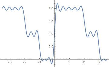
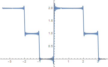
To compare the quality of Fourier approximations,
we plot partial sums with 10 and 50 terms, respectively:
curve = 5/4 - (1/Pi)*
Sum[Sin[k*Pi/2]*Cos[k*Pi*x/2]/k, {k, 1, 10}] - (1/Pi)*
Sum[(Cos[k*Pi/2] + (-1)^k - 2)*Sin[k*Pi*x/2]/k, {k, 1, 10}]
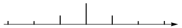
When the complex Fourier series is used to represent a periodic function, then the amplitude spectrum, sketched below, is two-sided. It consists of the points
\( \left( \frac{k\pi}{\ell} , \left\vert \alpha_k \right\vert \right) , \quad k= 0, \pm 1, \pm 2, \ldots \) that in our case become
\[
\left( 0, \frac{5}{4} \right) , \quad \left( \frac{k\pi}{2}, \frac{1}{2k\pi} \,\sqrt{\left( (-1)^k + \cos \frac{k\pi}{2} -2 \right)^2 + \sin^2 \frac{k\pi}{2}} \right) , \quad k=\pm 1, \pm 2, \ldots .
\]
a[k_] = (-1)^k + Cos[k*Pi/2] - 2
The two-sided amplitude spectrum of the function.
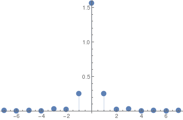
The power spectrum for
f is also two-sided, consisting of the points
\( \left( \frac{k\pi}{\ell} , \left\vert \alpha_k \right\vert^2 \right) , \quad k= 0, \pm 1, \pm 2, \ldots \) that in our case become
\[
\left( 0, \frac{5}{4} \right) , \quad \left( \frac{k\pi}{2}, \frac{1}{4k^2\pi^2} \,\left[ \left( (-1)^k + \cos \frac{k\pi}{2} -2 \right)^2 + \sin^2 \frac{k\pi}{2} \right] \right) , \quad k=\pm 1, \pm 2, \ldots .
\]
f[t_] = Piecewise[{{1, -2 < t < -1}, {0, -1 < t < 0}, {2, 0 < t < 2}}]
Note that here we used
Mathematica 's command
FourierCoefficient that gives the
k th coefficient in the Fourier series expansion of
f .
The two-sided power spectrum of the function.
■
The complex exponential Fourier form has the following advantages compared to the traditional trigonometric form:
only need to perform one integration;
a single exponential can be manipulated more easily than a sum of sinusoidal terms, and
it provides a logical transition into a further discussion of the Fourier Transform .
A signal's Fourier series spectrum
\( \alpha_k \) has interesting properties.
If f(t) is a real function, then \( \alpha_{-k} = \overline{\alpha_k} ; \)
if f(t) is an even function, then \( \alpha_{-k} = \alpha_k ; \) if f(t) is an odd function, then \( \alpha_{-k} = -\alpha_k , \) , and
the Fourier series obeys
Parseval's Theorem : \(
\int_0^T f^2 (t) \,{\text d}t = T\,\sum_k \left\vert \alpha_k \right\vert^2 .
\)
The following formula may be helpful for evaluating Fourier coefficients:
\begin{align*}
\int p(x)\, e^{ax}\,{\text d}x &= \frac{1}{a} \, e^{ax}\,\sum_{k=0}^n
\frac{(-1)^k}{a^k} \,{\texttt D}_x^k p(x) \qquad\quad \left( {\texttt D}_x =
\frac{\text d}{{\text d}x} \right)
\\
&= \frac{1}{a} \, e^{ax} \left[ p(x) - \frac{p' (x)}{a} + \frac{p'' (x)}{a^2}
- \cdots + (-1)^n \,\frac{p^{(n)} (x)}{a^n} \right] ,
\end{align*}
where
\( p(x) = b_n x^n + b_{n-1} x^{n-1} + \cdots + b_1 x + b_0 \) is a polynomial of degree
n .
Example 2: Fourier series for a fractional function
Example 2: \( f(x) = \frac{1-a\,\cos x}{1- 2a\,\cos x + a^2} , \) where real number a has absolute value less than 1: \( |a| <1 . \)
First, we substitute Euler's representation \( \cos x = \frac{1}{2}\,e^{{\bf j}x} + \frac{1}{2}\,e^{-{\bf j}x} . \)
instead of cos(x ).
Then
\[
f(x) = \frac{1 - \frac{a}{2} \left( e^{{\bf j}x} + e^{-{\bf j}x} \right)}{1 - a \left( e^{{\bf j}x} + e^{-{\bf j}x} \right) + a^2} = \frac{1}{2}\,\frac{2- a\, e^{{\bf j}x} - a\,e^{-{\bf j}x}}{\left( 1-a\,e^{{\bf j}x} \right) \left( 1-a\,e^{-{\bf j}x} \right)} .
\]
Since the numerator can be written as
\[
2- a\, e^{{\bf j}x} - a\,e^{-{\bf j}x} = 1- a\, e^{{\bf j}x} + 1 - a\, e^{-{\bf j}x} ,
\]
we simplify the given function as
\[
f(x) = \frac{1}{2}\,\frac{1- a\, e^{{\bf j}x} + 1 - a\, e^{-{\bf j}x}}{\left( 1-a\,e^{{\bf j}x} \right) \left( 1-a\,e^{-{\bf j}x} \right)} = \frac{1}{2}\,\frac{1}{1-a\,e^{-{\bf j}x}} + \frac{1}{2}\,\frac{1}{1-a\,e^{{\bf j}x}}
\]
Using the geometric series formula
\( \frac{1}{1-q} = \sum_{n\ge 0} q^n \) twice, first time with
\( q= a\,e^{-{\bf j}x} \) and second time with
\( q= a\,e^{{\bf j}x} , \) we obtain the required complex Fourier series:
\[
f(x) = \frac{1}{2}\,\sum_{n\ge 0} \left( a\,e^{-{\bf j}x} \right)^n + \frac{1}{2}\,\sum_{n\ge 0} \left( a\,e^{{\bf j}x} \right)^n = \frac{1}{2}\,\sum_{n\ge 0} a^n \, e^{-n{\bf j}x} + \frac{1}{2}\,\sum_{n\ge 0} a^n \, e^{n{\bf j}x} ,
\]
which we rewrite in a symmetric way
\[
f(x) = 1+ \frac{1}{2}\,\sum_{n\ge 1} a^n \, e^{n{\bf j}x} + \frac{1}{2}\,\sum_{n=-\infty}^{-1} a^{-n} \, e^{n{\bf j}x} .
\]
Next, we unite these two sums into one to obtain real trigonometric series:
\[
\frac{1-a\,\cos x}{1- 2a\,\cos x + a^2} = \sum_{n\ge 0} a^n \cos nx .
\]
■
Example 3: Fourier series for a periodic pulse function
Example 3: pulse function shown below
\[
\Pi (t,h,T) = \left\{
\begin{array}{ll}
1 , & \ x\in (0, h) \\
0 , & \ x\in (h,T)
\end{array}
\right. \qquad\mbox{on the interval } (0,T).
\]
The function is a pulse function with amplitude 1, and pulse width
h , and period
T . Using
Mathematica , we can define the pulse function in many ways; however, we demonstrate application of command
Which . The
Which command provides a logical expression that allows us to evaluate a function in only one statement like the one given in the equation, defining the pulse function. The "Which" command has the general form :
Which[condition1, value1, condition2, value2 ...]
The command will return the value that is true; let us see how this works in practice in an example of the pulse function:
PI[x_, h_, T_] := Which[0 < x < h, 1, h < x < T, 0]
We expand the pulse function into exponential Fourier series:
\[
\Pi (x,h,T) = \sum_{k=-\infty}^{\infty} \alpha_k e^{{\bf j}k2\pi x/T}, \qquad \alpha_k = \frac{1}{T} \,\int_0^h e^{-{\bf j}k2\pi x/T} \,{\text d}x = \frac{\bf j}{2k\pi} \left[ e^{-{\bf j}k2\pi h/T} -1 \right] , \quad k=0, \pm 1, \pm 2, \ldots .
\]
Note that the corresponding
k = 0 value α
0 =
h/T does not follow from the general formula directly. The above Fourier series defines the pulse functions at the points of discontinuity as the mean values from left and right:
\[
\Pi (0,h,T) = \Pi (h,h,T) = \frac{1}{2} = \frac{h}{T} + \sum_{k \ge 0} \frac{1}{k\pi} \, \sin \frac{2hk\pi}{T} \qquad\mbox{for any }h, t.
\]
We can also convert the complex Fourier form to a regular real trigonometric form:
\[
\Pi (x,h,T) = \frac{h}{T} + \sum_{k \ge 0} \frac{1}{k\pi} \left[ \sin \frac{2hk\pi}{T} \, \cos \frac{2\pi kx}{T} + 2\,\sin^2 \frac{k\pi h}{T} \,\sin \frac{2\pi kx}{T} \right] .
\]
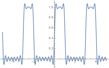
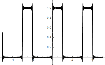
To compare the quality of Fourier approximations, we plot partial sums with 10 and 50 terms for particular numerical values
h = 1 and
T = 3: \)
pulse10 =
1/3 + (1/Pi)*Sum[(1/k)*(Sin[2*k*Pi/3]*Cos[2*Pi*k*x/3] +
2*(Sin[k*Pi/3])^2 *Sin[2*Pi*k*x/3]), {k, 1, 10}]
We can calculate Fourier coefficients directly:
a0 = 2/3;
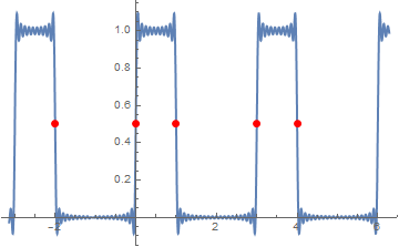
Then we check numerical values of the partial sum with 30 terms at the points of discontinuity:
N[fourier[30] /. x -> 1]
Out[23]= 0.496939
which is closed to the true value
\( \Pi (1,1,3)=1/2. \)
■
Example 4: Fourier series for a piecewise continuous function
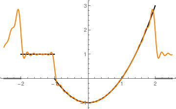
Example 4:
\[
f(x) = \begin{cases} 1, & \ \mbox {if } -2 < x < -1 , \\
x^2 -1, & \ \mbox {if } -1< x< 2 ,
\end{cases}
\]
Its Fourier coefficients are evaluated with the aid of
Mathematica :
f[x_] = Piecewise[{{1, -2 < x < -1}, {x^2 - 1, -1 < x < 2}}, 0]
1/4
Other coefficients we find by direct integration:
Simplify[Integrate[f[x]*Exp[-n*Pi*I*x/2], {x, -2, 2}]/4 , Assumptions -> {Element[n, Integers], Element[x, Reals]}]
((-1)^n (8 I (-1 + I^(3 n)) + 4 (2 + I^(3 n)) n \[Pi] +
I (2 + I^(3 n)) n^2 \[Pi]^2))/(2 n^3 \[Pi]^3)
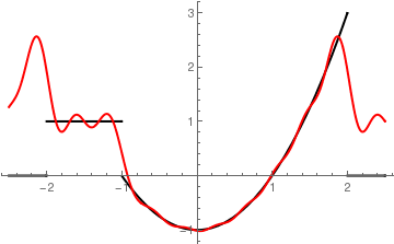
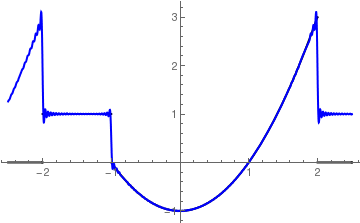
Now we build partial sums with
N = 10, 20, and 100 terms
F10[x_] = 1/4 + Simplify[Sum[ (((-1)^n (8 I (-1 + I^(3 n)) +
4 (2 + I^(3 n)) n \[Pi] +
I (2 + I^(3 n)) n^2 \[Pi]^2))/(2 n^3 \[Pi]^3))*Exp[n*Pi*I*x/2], {n, 1, 10}] +
Sum[ (((-1)^n (8 I (-1 + I^(3 n)) +
4 (2 + I^(3 n)) n \[Pi] +
I (2 + I^(3 n)) n^2 \[Pi]^2))/(2 n^3 \[Pi]^3))*Exp[n*Pi*I*x/2], {n, -10, -1}]]
and plot them
Plot[{f[x], F10[x]}, {x, -2.5, 2.5},
PlotStyle -> {{Thick, Black}, {Thick, Red}}]
Fourier approximation with 10 terms
Fourier approximation with 20 terms
Fourier approximation with 100 terms
■
Example 5: Fourier series for the Heaviside function
Example 5:
\[
H(x) = \begin{cases} 1, & \ \mbox {if } 0 < x < \ell , \\
0, & \ \mbox {if } -\ell < x< 0 .
\end{cases}
\]
Expanding the Heaviside function into the Fourier series
\[
H(x) = \mbox{P.V.} \sum_{k=-\infty}^{\infty} \alpha_k e^{k{\bf j} \pi x/\ell} = \lim_{N\to\infty} \sum_{k=-N}^{N} \alpha_k e^{k{\bf j} \pi x/\ell} ,
\]
where
\[
\alpha_k = \frac{1}{2\ell} \int_{0}^{\ell} e^{-k{\bf j} \pi x/\ell} \,{\text d} x = \frac{\bf j}{2k\pi} \left( 1 - e^{{\bf j}k\pi} \right)
\]
Integrate[Exp[k*I*Pi*x/L], {x, 0, L}]/2/L
-((I (-1 + E^(I k \[Pi])))/(2 k \[Pi]))
Since
\( e^{{\bf j}k\pi} = (-1)^k , \) , we get
\[
H(x) = \frac{1}{2} + \frac{2}{\pi} \sum_{k\ge 0} \frac{1}{2k+1}\,\sin \frac{\left( 2k+1 \right) \pi x}{\ell} .
\]
FourierSeries[HeavisideTheta[t], t, 3]
1/2 + (I E^(-I t))/\[Pi] - (I E^(I t))/\[Pi] + (I E^(-3 I t))/(
3 \[Pi]) - (I E^(3 I t))/(3 \[Pi])
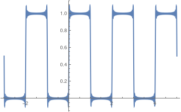
We check the series by plotting partial sums.
S20[x_] = 1/2 + (2/Pi)*Sum[Sin[(2*k + 1)*Pi*x]/(2*k + 1), {k, 0, 20}];
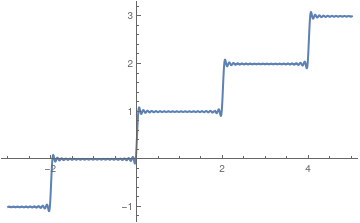
However, if you integrate Eq.\eqref{EqComplex.4} term-by-term, you will get
another Fourier series expansion
\[
h(x) = \frac{1}{2} + \frac{x\pi}{2\ell} + \frac{1}{\pi} \sum_{k\ge 1} \frac{1}{k}\,\sin \left( \frac{k\pi x}{\ell} \right) .
\]
Actually, the function
h (
x ) is a ladder function that coinside with the Heaviside function on the interval (−2ℓ, 2ℓ), as the folloing plots confirm:
SS20[x_] = 1/2 + (x/2) + (1/Pi)*Sum[Sin[k*Pi*x]/(k), {k, 1, 20}];
Fourier approximation with 20 terms of H(x)
Fourier approximation with 20 terms of h(x)
■
References
Stein, E.M., Shakarchi, R., Fourier Analysis: An Introduction, Princeton University Press, 2003. ISBN-13 : 978-0691113845
Return to Mathematica page main page (APMA0340) Part 1 Matrix Algebra Part 2 Linear Systems of Ordinary Differential Equations Part 3 Non-linear Systems of Ordinary Differential Equations Part 4 Numerical Methods Part 5 Fourier Series Part 6 Partial Differential Equations Part 7 Special Functions