Return to computing page for the second course APMA0340
Return to Mathematica tutorial for the first course APMA0330
Return to Mathematica tutorial for the second course APMA0340
Return to the main page for the course APMA0340
Return to the main page for the course APMA0330
Return to Part V of the course APMA0340
Introduction to Linear Algebra with Mathematica
Glossary
There are two known classes of functions for which the Euler--Fourier formulas for the coefficients can be simplified: even and odd. We define them as follows
Properties involving addition and subtraction:
- The sum of two even functions is even, and any constant multiple of an even function is even.
- The sum of two odd functions is odd, and any constant multiple of an odd function is odd.
- The difference between two odd functions is odd.
- The difference between two even functions is even.
- The sum of an even and odd function is neither even nor odd, unless one of the functions is equal to zero over the given domain.
Properties involving multiplication and division:
- The product of two even functions is an even function.
- The product of two odd functions is an even function.
- The product of an even function and an odd function is an odd function.
- The quotient of two even functions is an even function.
- The quotient of two odd functions is an even function.
- The quotient of an even function and an odd function is an odd function.
Properties involving composition:
- The composition of two even functions is even.
- The composition of two odd functions is odd.
- The composition of an even function and an odd function is even.
- The composition f ○ g = f(g) of any function f with an even function g is even (but not vice versa).
Other algebraic properties:
- Any linear combination of even functions is even. The set of even functions form a vector space over the real numbers ℝ. Similarly, any linear combination of odd functions is odd, and the odd functions also form a vector space over the reals. In other words, every function f(x) can be written uniquely as the sum of an even function and an odd function:
\[ f(x)=f_{\text{e}}(x)+f_{\text{o}}(x) , \]where\[ f_{\text{e}}(x)=\tfrac {1}{2} \left[ f(x)+f(-x) \right] , \]is even and\[ {\displaystyle f_{\text{o}}(x)={\tfrac{1}{2}}[f(x)-f(-x)]} \]is odd. For example, if \( f(x) = e^x , \) then its even part, fe, is cosh(x) and its odd part, fo, is sinh(x).
Basic calculus properties:
- The derivative of an even function is odd.
- The derivative of an odd function is even.
- The integral of an odd function from -A to +A is zero (where A is finite, and the function has no vertical asymptotes between -A and A): \( \int_{-A}^A f_{\text{o}}(x) \,{\text d}x = 0. \)
- The integral of an even function from -A to +A is twice the integral from 0 to +A (where A is finite, and the function has no vertical asymptotes between -A and A): \( \int_{-A}^A f_{\text{e}}(x) \,{\text d}x = 2 \int_0^A f_{\text{e}}(x) \,{\text d}x . \) This also holds true when A is infinite, but only if the integral converges).
Series properties:
- The Maclaurin series of an even function includes only even powers.
- The Maclaurin series of an odd function includes only odd powers.
- The Fourier series of a periodic even function includes only cosine terms.
- The Fourier series of a periodic odd function includes only sine terms.
Fourier Sine Series and Fourier Cosine Series
If a function f(x) is defined on a finite interval (𝑎, b), it can be extended periodically in three different ways:
- Periodically with period \( T= b-a . \) This can be achieved by expanding f into regular real Fourier series:
\begin{equation} \label{EqEven.1} f(x) \sim \frac{a_0}{2} + \sum_{n\ge 1} \left[ a_n \cos \left( \frac{2\pi nx}{T} \right) + b_n \sin \left( \frac{2\pi nx}{T} \right) \right] , \qquad a_n = \frac{2}{T} \int_T f(x) \,\cos \frac{2\pi nx}{T}\,{\text d}x , \quad b_n = \frac{2}{T} \int_T f(x) \,\sin \frac{2\pi nx}{T}\,{\text d}x ; \quad n=0,1,2,\ldots ; \end{equation}or complex Fourier series:\begin{equation} \label{EqEven.2} f(x) \sim \mbox{P.V.} \sum_{n=-\infty}^{+\infty} \hat{f}(n)\, e^{2{\bf j}\pi nx/T} , \qquad \hat{f}(n) = \frac{1}{T} \int_T f(x)\, e^{-2{\bf j}\pi nx/T} \,{\text d}x , \quad n=0, \pm 1, \pm 2, \ldots . \end{equation}
- Periodically with period \( T= 2(b-a) = 2\ell , \) with ℓ = b−𝑎, by making the extension an even function. This can be achieved upon expanding f into Fourier cosine series:
\begin{equation} \label{EqEven.3} f(x) \sim \frac{a_0}{2} + \sum_{n\ge 1} a_n \cos \frac{n\pi x}{\ell} , \qquad a_n = \frac{2}{\ell} \int_{0}^{\ell} f(x) \,\cos \frac{n\pi x}{\ell}\,{\text d}x ; \quad n=0,1,2,\ldots . \end{equation}
-
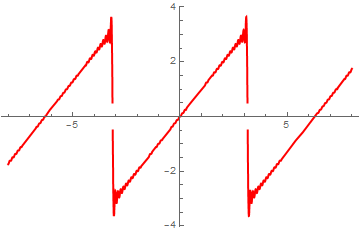
Periodically with period \( T= 2(b-a) = 2\ell \) by making the extension an odd function. This can be achieved upon expanding f into Fourier sine series:
\begin{equation} \label{EqEven.4} f(x) \sim \sum_{n\ge 1} b_n \sin \frac{n\pi x}{\ell} , \qquad a_n = \frac{2}{\ell} \int_{0}^{\ell} f(x) \,\sin \frac{\pi nx}{\ell}\,{\text d}x ; \quad n=1,2,\ldots . \end{equation}
- If bk = o(1/k), the cosine expansion \eqref{EqEven.6} converges at x = 0 to sum 0;
- If bk = O(1/k) and f is continuous at 0, then cosine expansion \eqref{EqEven.6} converges uniformly at x = 0;
- If bk = O(1/k) and f is continuous in a neighborhood 0 ≤ x ≤ δ, then cosine expansion \eqref{EqEven.6} converges uniformly in [0, δ].
-
We know that the signum function has the Fourier expansion
\[ \mbox{sign}(x) = \frac{4}{\pi} \sum_{\nu \ge 1} \frac{\sin \left( 2\nu -1 \right) x}{2\nu -1} = \frac{2}{\pi{\bf j}} \sum_{\nu \ge 1} \frac{1}{2\nu -1}\,e^{{\bf j} \left( 2\nu -1 \right) x} . \]Since expansion \eqref{EqEven.6} is the product of expansion \eqref{EqEven.5} and the signum function, the conclusion follows from Theorem 17 of section.
-
If
\[ | s_n | \le \epsilon , \qquad |t_n | \le 1, \qquad |c_n | \le 1/|n| \]for all n, then | Sn | ≤ Aϵ is an absolute constant.
Suppose first that f(+0) = 0; then the partial sums sn of \eqref{EqEven.5} converges uniformly at x = 0. Thus, omitting if necessary the first few terms in \eqref{EqEven.5}, we have | sn | ≤ ϵ for |x| ≤ η. Since the partial sum,s of the Fourier series S[sign] are uniformly bounded, it follows that the partial sums Sn(x) of \eqref{EqEven.6} satisfy | Sn(x) | ≤ Aϵ for |x| ≤ η, and since the contribution to Sn(x) of the omitted terms converges uniformly to a limit, part (ii) is established. The case f(+0) ≠ 0 is reduced to the preceding one by subtracting f(+0) S[sign] from series \eqref{EqEven.5}.
- At every x interior to (0, π), the uniform convergence of series \eqref{EqEven.5} implies that of \eqref{EqEven.6}. Hence, using part (ii), series \eqref{EqEven.6} converges uniformly at every point of the closed interval [0, δ], and so converges uniformly in that interval.
if 𝑎k = O(1/k), f is continuous at x = 0 and f(0) = 0, then \eqref{EqEven.5} converges uniformly at x = 0.
A similar extension holds for part (iii). The proofs remain unchanged.
We demonstrate all these approaches in the following examples.
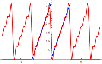
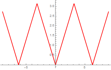
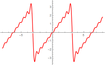
Example 1: We start with a simple function, which is of saw-tooth type: \( g(t) = t \) on the interval (0, π ) that we first extend periodically with period π and then expand it into regular Fourier series:
ak = Simplify[ Integrate[t*Cos[k*t], {t, 0, Pi}, Assumptions -> Element[k, Integers]]/Pi + Integrate[(t + Pi)*Cos[k*t], {t, -Pi, 0}, Assumptions -> Element[k, Integers]]/Pi ]
bk = Simplify[ Integrate[t*Sin[k*t], {t, 0, Pi}, Assumptions -> Element[k, Integers]]/Pi + Integrate[(t + Pi)*Sin[k*t], {t, -Pi, 0}, Assumptions -> Element[k, Integers]]/Pi ]
fourier[m_] := Pi/2 + Sum[ak*Cos[k*t] + bk*Sin[k*t], {k, 1, m}]
bn = Assuming[Element[n, Integers], Integrate[f[x]*Sin[n*x], {x, -Pi, Pi}]/Pi]
Bn = 2*Integrate[t*Sin[2*n*t], {t, 0, Pi}]/Pi
Plot[{f[t], fourier[50]}, {t, -8, 8}, PlotStyle -> {{Thick, Blue}, {Thick, Red}}]
 |
 |
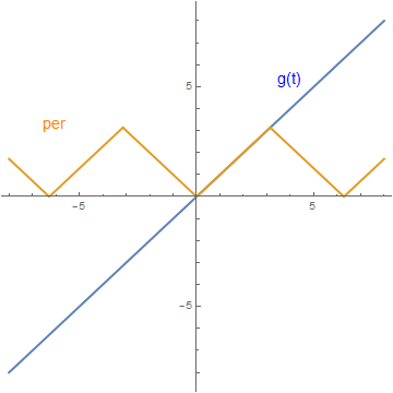
g[t_] = t
per = periodicExtension[g]
a = Plot[{g[t], per}, {t, -8, 8}, PlotStyle -> Thick, AspectRatio -> 1]
Show[a, Graphics[{Text[Style["g(t)", FontSize -> 14, Blue], {4, 5.3}], Text[Style["per", FontSize -> 14, Orange], {-6, 3.3}]}]]
ak = Simplify[Integrate[t*Cos[k*t], {t, 0, Pi}]*2/Pi ]
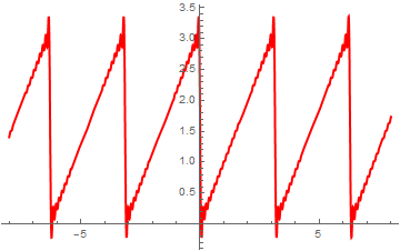
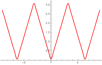
even[m_] := Pi/2 + Sum[ak*Cos[k*t], {k, 1, m}]
Plot[{even[50]}, {t, -8, 8}, PlotStyle -> {Thick, Red}]
 |
 |
Plot[odd[10], {t, -8, 8}, PlotStyle -> {Thick, Red}]
 |
 |
FourierSinCoefficient[ expr , t, n] gives the n-th coefficient in the Fourier sine series expansion of expr.
FourierCosCoefficient[ expr , t, n] gives the n-th coefficient in the Fourier cosine series expansion of expr.
FourierCosSeries[expr, t , n] gives the n-order Fourier cosine series expansion of expr in t.
FourierSinSeries[expr, t , n] gives the n-order Fourier sine series expansion of expr in t.
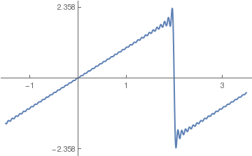
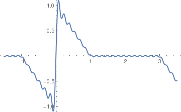
Similarly, we get sine Fourier series (Gibbs overshoot and undershoot are given explicitly):
Plot[%, {x, -1.5, 3.5}, PlotStyle -> Thick, Ticks -> {{-1, 1, 3}, {2.358, -2.358}}]
|
Finally, we demonstrate animation for Fourier series approximations.
s[x_, m_] = Pi/2 - Sum[Sin[2*n*x]/n, {n, 1, m}];
animation = Table[Plot[s[x, m], {x, -0.1, Pi + 0.1}, PlotRange -> {0, 3.2}, PlotStyle -> Thickness[0.008], PlotLabel -> "Fourier approximation depends on " <> ToString[m] <> " terms"], {m, 0, 100, 2}]; Export["saw.gif", animation, "AnimationRepetitions" -> 200] |
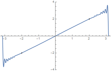
Example 2: Let us consider the function f(x) = x, assuming it is defined in the interval [-π , π ].
a0 = (1/Pi)* Integrate[f[x], {x, −Pi, Pi}];
an = (1/Pi)* Integrate[f[x]*Cos[n*x], {x, −Pi, Pi}, Assumptions -> Element[n, Integers]];
bn = (1/Pi)* Integrate[f[x]*Sin[n*x], {x, −Pi, Pi}, Assumptions -> Element[n, Integers]];
Print[{a0, an, bn}]
Plot[fourier[10], {x, -Pi, Pi}, Epilog -> Point[{{2, 2}, {-2, -2}}], PlotStyle -> {Thick, Black}]
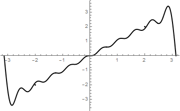
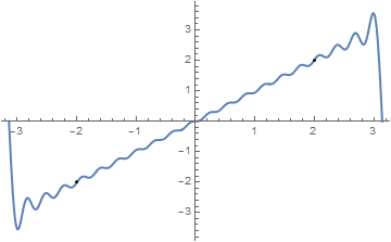
Plot[fourier[50], {x, -Pi, Pi}, Epilog -> Point[{{2, 2}, {-2, -2}}], PlotStyle -> Thick]
 |
 |
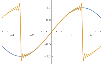
Example 3: Since the function sin(x/2) is an odd function on the interval [-π,π], we can expand it into sine Fourier series explicitly:
Plot[{Sin[x/2], F[x]}, {x,-5,5}, PlotStyle->Thick]
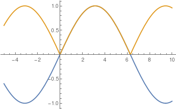
We can also expand the given function sin(x/2) into cosine Fourier series by expanding it to negative semi-axis in even way. First, we calculate Fourier coefficients:
an= Simplify[2/Pi*Integrate[Sin[x/2]*Cos[n*x], {x,0,Pi}]];
(4 - 8 n Sin[n \[Pi]])/(\[Pi] - 4 n^2 \[Pi])
Plot[{Sin[x/2], F[x]}, {x,-5,10}, PlotStyle->Thick]
FourierCosSeries[f[x], x, 3]
Cos[2 x] Sin[1]^2)/\[Pi] + (4 Cos[3 x] Sin[3/2]^2)/(9 \[Pi])
Plot[coscurve5Pi, {x, -1.5, 3.5}]
then with 50 terms:
Plot[coscurve50Pi, {x, -1.5, 3.5}]
Then we repeat these calculation for cosine series on the interval of length 2:
Plot[%, {x, -1.5, 3.5}]
FourierSinSeries[f[x], x, 25, FourierParameters -> {1, Pi/2}];
Plot[%, {x, -1.5, 3.5}, PlotStyle->Thick, PlotRange->{-1.1,1.1}]
Example 5A: We are going to prove the well-known trigonometric identity:
L=Pi
a0 = 2/L*Integrate[f[x], {x, 0, L}]
ak = 2/L*Integrate[f[x]*Cos[x*k*Pi/L], {x, 0, L}]
However, we notice that cos² is actually a periodic function with period π, so we can find its cosine Fourier series with 2 L = π:
a0 = 2/L*Integrate[f[x], {x, 0, L}]
ak = 2/L*Integrate[f[x]*Cos[x*k*Pi/L], {x, 0, L}]
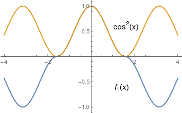
Now we consider another function that coincides with cos²x on the interval (-π,π):
a = Plot[{F[x], (Cos[x])^2}, {x, -4, 4}, PlotStyle -> Thick]
text1 = Graphics[ Text[Style["\!\(\*SubscriptBox[\(f\), \(1\)]\)(x)", FontSize -> 14, Black], {1.4, -0.6}]]
text2 = Graphics[ Text[Style["\!\(\*SuperscriptBox[\(cos\), \(2\)]\)(x)", FontSize -> 14, Black], {1.6, 0.6}]]
Show[a, text1, text2]
Example 5B: Now we derive the identity:
L = Pi a0 = 2/L*Integrate[g[x], {x, 0, L}]
ak = 2/L*Integrate[g[x]*Cos[x*k*Pi/L], {x, 0, L}]
a2 = 2/L*Integrate[g[x]*Cos[x*2*Pi/L], {x, 0, L}]
a3 = 2/L*Integrate[g[x]*Cos[x*3*Pi/L], {x, 0, L}]
1/4
a0 = 2/L*Integrate[g[x], {x, 0, L}]
ak = 2/L*Integrate[g[x]*Cos[x*k*2], {x, 0, L}]
Plot[{Callout[SF10[x], "Fourier 10", LabelStyle -> Directive[Purple, Bold]], Callout[Sin[1/x], "Exact"]}, {x, 0, 1}, PlotStyle -> {{Thick, Orange}, {Thick, Blue}}]
Plot[{Callout[SF10[x], "Fourier 10", LabelStyle -> Directive[Purple, Bold]], Callout[Sin[1/x], "Exact"]}, {x, 0.001, 0.1}, PlotStyle -> {{Thick, Orange}, {Thick, Blue}}]
|
|
|
Then we repeat calculations with 100 terms:
Plot[{Callout[SF100[x], "Fourier 100", LabelStyle -> Directive[Purple, Bold]], Callout[Sin[1/x], "Exact", LabelStyle -> Directive[Blue, Bold]]}, {x, 0.001, 1}, PlotStyle -> {{Thick, Orange}, {Thick, Blue}}]
Plot[{Callout[SF100[x], "Fourier 100", LabelStyle -> Directive[Purple, Bold]], Callout[Sin[1/x], "Exact", LabelStyle -> Directive[Blue, Bold]]}, {x, 0.001, 0.1}, PlotStyle -> {{Thick, Orange}, {Thick, Blue}}]
|
|
|
We apply Cesàro summation.
Plot[{Callout[CF100[x], "Cesaro 100", LabelStyle -> Directive[Red, Bold]], Callout[Sin[1/x], "Exact", LabelStyle -> Directive[Blue, Bold]]}, {x, 0.005, 1}, PlotStyle -> {{Thick, Red}, {Thick, Blue}}]
Plot[{Callout[CF100[x], "Cesaro 100", LabelStyle -> Directive[Red, Bold]], Callout[Sin[1/x], "Exact", LabelStyle -> Directive[Blue, Bold]]}, {x, 0.005, 0.1}, PlotStyle -> {{Thick, Red}, {Thick, Blue}}]
|
|
|
Finally, we take 1000 terms:
Plot[{Callout[SF1000[x], "Fourier 1000", LabelStyle -> Directive[Purple, Bold]], Callout[Sin[1/x], "Exact", LabelStyle -> Directive[Blue, Bold]]}, {x, 0.005, 1}, PlotStyle -> {{Thick, Orange}, {Thick, Blue}}]
Plot[{Callout[SF1000[x], "Fourier 1000", LabelStyle -> Directive[Purple, Bold]], Callout[Sin[1/x], "Exact"]}, {x, 0.005, 0.02}, PlotStyle -> {{Thick, Orange}, {Thick, Blue}}]
|
|
|
Cesàro summation gives:
|
|
|
We compare which of two approximations, Fourier or Cesàro, gives a better approximation using their graphical outputs. Since human's eyes have a resolution of about 5%, it gives us only qualitative conclusion. Working with 1000-term approximations, we conclude that the Cesàro approximation is accurate enough after x > 0.1. When x → 0, Cesàro approximation tends to zero and does not match the function. On the other hand, Fourier approximation gives a reasonable accuracy forx > 0.04, but exhibits the Gibbs phenomenon at the boundary x = 1,
|
|
|
■
Return to Mathematica page
Return to the main page (APMA0340)
Return to the Part 1 Matrix Algebra
Return to the Part 2 Linear Systems of Ordinary Differential Equations
Return to the Part 3 Non-linear Systems of Ordinary Differential Equations
Return to the Part 4 Numerical Methods
Return to the Part 5 Fourier Series
Return to the Part 6 Partial Differential Equations
Return to the Part 7 Special Functions