Preface
This section presents examples of electric circuits and corresponding differential equations.
Return to computing page for the second course APMA0340
Return to Mathematica tutorial for the first course APMA0330
Return to Mathematica tutorial for the second course APMA0340
Return to the main page for the first course APMA0330
Return to the main page for the second course APMA0340
Return to Part II of the course APMA0340
Introduction to Linear Algebra with Mathematica
Glossary
Electric Circuits
We show interconnection between electric circuits and differential equations used to model them in a series of examples. We start with the most simple example when resistor , inductor , and capacitor are connected in series across a voltage supply, the circuit so obtained is called series RLC circuit. A good introduction to the subject could be found on the web . The phasor diagram of series RLC circuit is drawn by combining the phasor diagram of resistor, inductor and capacitor. Before doing so, one should understand the relationship between voltage and electric current in case of resistor, capacitor and inductor.
Example 1: Consider RCL circuit in series.
- Derive the time response of an RLC circuit due to a varying signal.
- Describe the individual components of the RLC circuit.
- By Ohm's
Law, the voltage across a resistor is the current passing
through it multiplied by its resistance in ohms.
\[ V_R (t) = R \cdot i(t) . \]
- The voltage across a capacitor is less intuitive. Physically, a basic capacitor is just two metal plates with some conductive material across it. The voltage across it is best described by this equation C*V=Q. Where the dQ/dt is the rate of charge passing through the capacitor, or the current i(t). Therefore, the voltage across a capacitor is the total charge passing through the capacitor scaled by a capacitor constant. (Helpful additional reading about the capacitor: http://hyperphysics.phy-astr.gsu.edu/hbase/electric/pplate.html )
- An inductor is just a coil of wire. The coiling of the wire produces some interesting electric field properties that make
the answer tot he voltage across it not so trivial. With a current source that does not vary with time, the inductor will
act as a short circuit, so the voltage across it will be zero. But if current across the inductor changes, the inductor's
electric field will resist the change The voltage across an inductor can be described by V=L*di/dt. In words, the
voltage across an inductor is proportional to its electric field and the rate of change of current through it. (Helpful
addition reading about the inductor: https://www.allaboutcircuits.com/textbook/direct-current/chpt-15/inductors-and-
calculus/)
\[ V_L (t) = L \cdot \frac{\text d}{{\text d}t}\, i(t) . \]
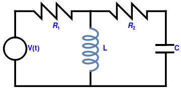
Example 2: Let us consider a two-loop circuit:
|
resistor1 =
Graphics[{Thickness[0.01],
Line[{{-30, 12}, {-25, 12}, {-23, 10}, {-23, 14}, {-19,
10}, {-19, 14}, {-15, 10}, {-15, 12}, {-10, 12}}]},
PlotLabel -> Subscript[R, 1], Ticks -> None, Axes -> False];
resistor2 = Graphics[{Thickness[0.01], Line[{{-10, 12}, {-5, 12}, {-3, 10}, {-3, 14}, {1, 10}, {1, 14}, {5, 10}, {5, 12}, {10, 12}}]}, PlotLabel -> Subscript[R, 2], Ticks -> None, Axes -> False]; coil = ParametricPlot[{2*Sin[t*3] - 10, 1*Cos[t*3 + Pi] + 1*t - 3}, {t, 0, 3*Pi}, PlotLabel -> "L", Ticks -> None, Axes -> False, ImageSize -> Tiny, PlotStyle -> {Thickness[0.01]}]; l1 = Graphics[{Thickness[0.01], Line[{{-30, -1}, {-30, -8}, {10, -8}}]}]; l2 = Graphics[{Thickness[0.01], Line[{{-30, 5}, {-30, 12}}]}]; l3 = Graphics[{Thickness[0.01], Line[{{-10, 12}, {-10, 7.5}}]}]; l4 = Graphics[{Thickness[0.01], Line[{{-10, -8}, {-10, -4}}]}]; l5 = Graphics[{Thickness[0.01], Line[{{10, 12}, {10, 3}, {8, 3}, {12, 3}}]}]; l6 = Graphics[{Thickness[0.01], Line[{{10, -8}, {10, 1}, {8, 1}, {12, 1}}]}]; c1 = Graphics[{Thickness[0.01], Circle[{-30, 2}, 3]}]; txtC = Graphics[ Text[Style["C", Bold, FontSize -> 14, Blue], {13, 2}]]; txtV = Graphics[ Text[Style["V(t)", Bold, FontSize -> 14, Blue], {-25, 2}]]; txtL = Graphics[ Text[Style["L", Bold, FontSize -> 14, Blue], {-6, 2}]]; txtR1 = Graphics[ Text[Style[Subscript[R, 1], Bold, FontSize -> 14, Blue], {-19, 8}]]; txtR2 = Graphics[ Text[Style[Subscript[R, 2], Bold, FontSize -> 14, Blue], {1, 8}]]; Show[l1, l2, l3, l4, l5, l6, c1, resistor1, resistor2, coil, txtC, txtV, txtL, txtR1, txtR2] |
|
| Two-loop circuit. | Mathematica code |
We apply Kirchoff's voltage law (KVL) to each loop. The KVL deals with the conservation of energy around a closed circuit path. This voltage law states that for a closed loop series path the algebraic sum of all the voltages around any closed loop in a circuit is equal to zero. Since the choice of direction of current is arbitrary, we consider its direction as clockwise in every loop. As charge carriers flowing through a circuit pass though a component, they either gain or lose electrical energy, depending upon the component.
The left loop has three elements: a voltage source, V(t) = 127 sin(120πt and two passive elements: resitor R1 = 10 Ω and the coil (inductor) with inductance L = 0.1 H. The right loop consists again of the same coil, another resitor R2 = 20 Ω and capacitor with capacitance C = 1 mF = 0.001 F. Then for the left loop, we get
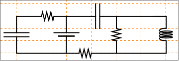
Example 3: Consider a three-loop circuit of a first order, given that each loop will contain only one energy storage element (capacitor or inductor) in addition to resistors. The capacitor current-voltage relationship, \( i = C\,\frac{{\text d}V}{{\text d}t} \) and inductor current-voltage relationship \( V = L\,\frac{{\text d}i}{{\text d}t} \) are first order differential equations. Ohm’s Law, i = V R and Kirchhoff’s Voltage Law, which defines the conservation of energy around a closed loop.
ap[l_ : 1] := Line[l {{{0, 0}, {1/3, 0}}, {{2/3, 0}, {1, 0}}}] resistor[l_ : 1, n_ : 3] := Line[Table[{i l/(4 n), 1/3 Sin[i Pi/2]}, {i, 0, 4 n}]]
coil[l_ : 1, n_ : 3] := Module[{ scale = l/(5/16 n + 1/2), pts = {{0, 0}, {0, 1}, {1/2, 1}, {1/2, 0}, {1/2, -1}, {5/ 16, -1}, {5/16, 0}} }, Append[Table[ BezierCurve[scale Map[{d 5/16, 0} + # &, pts]], {d, 0, n - 1}], BezierCurve[scale Map[{5/16 n, 0} + # &, pts[[1 ;; 4]]]]]]
capacitor[l_ : 1] := {gap[l], Line[l {{{1/3, -1}, {1/3, 1}}, {{2/3, -1}, {2/3, 1}}}]}
battery[l_ : 1] := {gap[ l], {Rectangle[l {1/3, -(2/3)}, l {1/3 + 1/9, 2/3}], Line[l {{2/3, -1}, {2/3, 1}}]}}
contact[l_ : 1] := {gap[l], Map[{EdgeForm[Directive[Thick, Black]], FaceForm[White], Disk[#, l/30]} &, l {{1/3, 0}, {2/3, 0}}]}
Options[display] = {Frame -> True, FrameTicks -> None, PlotRange -> All, GridLines -> Automatic, GridLinesStyle -> Directive[Orange, Dashed], AspectRatio -> Automatic};
display[d_, opts : OptionsPattern[]] := Graphics[Style[d, Thick], Join[FilterRules[{opts}, Options[Graphics]], Options[display]]]
at[position_, angle_ : 0][obj_] := GeometricTransformation[obj, Composition[TranslationTransform[position], RotationTransform[angle]]]
label[s_String, color_ : RGBColor[.3, .5, .8]] := Text@Style[s, FontColor -> color, FontFamily -> "Geneva", FontSize -> Large]; display[{ capacitor[] // at[{0, 0}, Pi/2], connect[{{0, 1}, {0, 2}, {2, 2}}], resistor[] // at[{2, 2}], connect[{{3, 2}, {4, 2}, {4, 1}}], battery[] // at[{4, 0}, Pi/2], connect[{{4, 0}, {4, -1}, {0, -1}, {0, 0}}], connect[{{4, 2}, {6, 2}}], capacitor[] // at[{6, 2}], connect[{{7, 2}, {8, 2}}], connect[{{8, 2}, {8, 1}}], resistor[] // at[{8, 0}, Pi/2], connect[{{8, 0}, {8, -1}, {6, -1}}], resistor[] // at[{5, -1}], connect[{{5, -1}, {4, -1}}], connect[{{8, 2}, {12, 2}}], connect[{{11, 2}, {12, 2}, {12, 1}}], coil[] // at[{12, 0}, Pi/2], connect[{{12, 0}, {12, -1}, {8, -1}}]}]
| Unit Name | Ubit Symbol | Quantity |
| Ampere (amp) | A | Electric current (I) |
| Volt | V |
Voltage (V, E) Electromotive force (E) Potential difference (Δφ) |
| Ohm | Ω | Resistance (R) |
| Watt | W | Electric power (P) |
| Farad | F | Capacitance (C) |
| Henry | H | Inductance (L) |
| Coulomb | C | Electric charge (Q) |
| Joule | J | Energy (E) |
| Tesla | T | Magnetic field (B) |
| Weber | Wb | Magnetic flux (Φm) |
| Hertz | Hz | Frequency (f) |
Return to Mathematica page
Return to the main page (APMA0340)
Return to the Part 1 Matrix Algebra
Return to the Part 2 Linear Systems of Ordinary Differential Equations
Return to the Part 3 Non-linear Systems of Ordinary Differential Equations
Return to the Part 4 Numerical Methods
Return to the Part 5 Fourier Series
Return to the Part 6 Partial Differential Equations
Return to the Part 7 Special Functions