Return to computing page for the second course APMA0340
Return to Mathematica tutorial for the first course APMA0330
Return to Mathematica tutorial for the second course APMA0340
Return to the main page for the first course APMA0330
Return to the main page for the second course APMA0340
Return to Part I of the course APMA0340
Introduction to Linear Algebra with Mathematica
Glossary
Chua's circuits

Many physical devices are modeled in such a way that the equations defining the system have \( \mathbb{Z}_2 \)-symmetry (invariance under the change of the sign in the state variables). In these systems, the origin is always an equilibrium point. Its simple, well arranged and transparent form expressed as a compact set of first-order ordinary differential equations (ODE) is also very convenient for modeling chaotic systems considered as determined systems exhibiting complex and unpredictable behavior.
There is no generally accepted definition of chaotic phenomena. Roughly speaking, a chaotic system is one that is deterministic but at the same time exhibits irregular, or random, behavior. A distinctive and readily observable property of chaotic systems is sensitive dependence on initial conditions: the trajectories starting from two arbitrarily close points diverge at an exponential rate and become uncorrelated in a short period of time. Chaos, or strange behavior, is currently one of the most exciting areas in the research of nonlinear systems.
The Chua circuit was invented in the fall of 1983 by the American electrical engineer and computer scientist Leon Ong Chua (born in 1936) in response to two unfulfilled quests among many researchers on chaos concerning two wanting aspects of the Lorenz equations (Lorenz, 1963). The first quest was to devise a laboratory system which can be realistically modeled by the Lorenz equations in order to demonstrate chaos is a robust physical phenomenon, and not merely an artifact of computer round-off errors. The second quest was to prove that the Lorenz attractor, which was obtained by computer simulation, is indeed chaotic in a rigorous mathematical sense. The existence of chaotic attractors from the Chua circuit had been confirmed numerically by Matsumoto (1984), observed experimentally by Zhong and Ayrom (1985), and proved rigorously in (Chua, et al, 1986). The basic approach of the proof is illustrated in a guided exercise on Chua’s circuit in the well-known textbook by Hirsch, Smale and Devaney (2003).
There are known three popular Chua's circuits presented in the following figures.
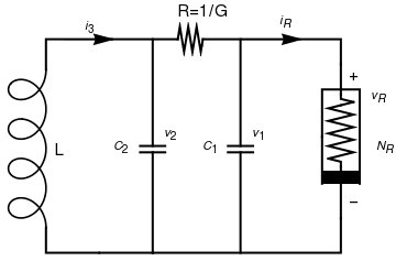
A basic Chua circuit consists of two capacitors C1 and C2 and the the inductor L, connected with so called Chua diod. Capacitors and inductors are called passive elements because they do not need a power supply e.g., battery). Interconnection of passive elements always leads to trivial dynamics, with all element voltages and currents tending to zero. The simplest circuit that could give rise to oscillatory or chaotic waveforms must include at least one locally active nonlinear element, powered by a battery, such as the Chua diode characterized by a current vs. voltage nonlinear function \( i_R = g \left( v_R \right) , \) whose slope must be negative somewhere on the curve. Such an element is called a locally active resistor. Although the function may assume many shapes, the original Chua circuit specifies the 3-segment piecewise-linear odd-symmetric characteristic:
\[ g\left( v_R \right) = \begin{cases} m_1 v_R + m_1 - m_0 , & \ \mbox{ if } v_R \le -1 , \\ m_0 v_R , & \ \mbox{ if } -1 \le v_R \le 1 , \\ m_1 v_R + m_0 - m_1 , & \ \mbox{ if } 1 \le v_R , \end{cases} \] where the coordinate of the two symmetric breakpoints are normalized, without loss of generality, to $v_R = \pm 1$.They can be modeled by the following dimensionless form of Chua's equa- tions
One of the reasons of the popularity of the Chua's circuit is due to the fact that it can generate a large variety of complex dynamics, and convoluted bifurcations, from a simple model in the form of a three-dimensional autonomous piecewise linear ordinary differential equation (flow).
It should be noted that instead of such piecewise function, cubic function can be implemented as well:
We consider first the original (noncanonical) Chua's circuit.
Many paradigms of chaotic systems modeling the main features of chaotic dynamics with only a few nonlinear equations, e.g. the Duffing equations, the Lorenz system, the Rössler system, Chua's equations, etc., are already known. Among all these paradigms is the Chua's model, i.e. Chua's equations and the corresponding Chua's circuits, that is of unique significance and for several reasons represents a milestone in the research on chaos theory and application. In comparison with the previous paradigms, Chua's model has the following advantages [Liao & Chen, 1998]. The Chua's equation is a model of one of the simplest electronic circuits, exhibiting a wide range of complex dynamical behaviors. Let us consider the Chua's equation with a cubic nonlinearity (see [Pivka et al., 1996]):
- References for Chua's circuit
- Bilotta, Eleonora and Pantano, Pietro, A Gallery of Chua Attractors, World Scientific Series on Nonlinear Science Series A: Volume 61, 2008, https://doi.org/10.1142/6720
- Chaotic behavior of Chuas circuit
- Chua, Leon, Chua circuit, (2007), Scholarpedia, 2(10):1488. Chua circuit, Wikipedia
- Chua, Leon, The Genesis of Chua's Circuit,
- Choi, Insook, A chaotic oscillator as a musical signal generator in an interactive performance system, Journal of New Music Research, doi: 10.1080/09298219708570715
- Hirsch, M. W., Smale, S. and Devaney, R. L., Differential Equations, Dynamical Systems & An Introduction to Chaos, 2003, Second Edition, Elsevier Academic Press, Amsterdam.
- Huang, S, Pivka, L, Wu, C W, and Franz, M., Chua's equation with cubic nonlinearity
- Liao, T. and Chen, F. Control of Chua's circuit with a cubic nonlinearity via nonlinear linearization technique, Circuits Systems Signal Process, 1998, Vol. 17, No. 6, pp. 719--731.
- Lorenz, E. (1963) Deterministic flow, Journal of Atmospheric Science, 20 : 130-141.
- Madan, R. N. (ed.) Chua's Circuit: A Paradigm for Chaos, 1993, (World Scientific, Singapore).
- Matsumoto, T. (1984) A Chaotic attract or from Chua’s Circuit, IEEE Transaction on Circuits and Systems, 31 : 1055-1058.
- Mira, C., Chua's circuit and the qualitative theory of dynamical systems
- Pivka, L., Wu, C. W. & Huang, A. [1996] "Lorenz equation and Chua's equation," International Journal of Bifurcation and Chaos, 6(12B), 2443--2489.
- Pospisil J, Kolka Z, Horska J, and Brzobohaty J, Simplest ODE equivalents of Chua's equations, International Journal of Bifurcation and Chaos, Vol. 10, No. 1 (2000) 1--23.
- Chua circuit Scholarpedia
- Shilnikov, L. P. "Chua's circuit: rigorous results and future problems", International Journal of Bifurcation and Chaos, Vol. 4(3), pp. 489-519, 1994.
- Siderskiy, Valentin, Matlab simulation.
- J. C. Sprott, Chaos and Time-Series Analysis, Oxford University Press, 2003.
- Tielo-Cuautle, E. and Munoz-Pacheco, J.M., Numerical Simulation of Chua's Circuit Oriented to Circuit Synthesis, International Journal of Nonlinear Sciences and Numerical Simulation, 8(2):249-256 · January 2007; doi: 10.1515/IJNSNS.2007.8.2.249
- Zhong, G.-Q., Implementation of Chua's Circuit with a Cubic Nonlinearity, IEEE Transactions on Circuits and Systems, 1994, Vol. 41, No. 12, pp. 934--941.
- Zhong, G.-Q. and Ayrom, F. [1985] Experimental confirmation of chaos from Chua's circuit, International Journal of Circuit Theory and Applications, 1985, Vol. 13, pp. 93--98. https://doi.org/10.1002/cta.4490130109
- Zhong, G.-Q., Man, K.-F., and Chen, G., A systematic approach to generating n-scroll attractors, International Journal of Bifurcation and Chaos, Vol. 12, No. 12 (2002) 2907--2915.
- Python(x,y)
Return to Mathematica page
Return to the main page (APMA0340)
Return to the Part 1 Matrix Algebra
Return to the Part 2 Linear Systems of Ordinary Differential Equations
Return to the Part 3 Non-linear Systems of Ordinary Differential Equations
Return to the Part 4 Numerical Methods
Return to the Part 5 Fourier Series
Return to the Part 6 Partial Differential Equations
Return to the Part 7 Special Functions