Preface
This section studies some first order nonlinear ordinary differential equations describing the time evolution (or “motion”) of those hamiltonian systems provided with a first integral linking implicitly both variables to a motion constant. An application has been performed on the Lotka--Volterra predator-prey system, turning to a strongly nonlinear differential equation in the phase variables.
Return to computing page for the first course APMA0330
Return to computing page for the second course APMA0340
Return to Mathematica tutorial for the first course APMA0330
Return to Mathematica tutorial for the second course APMA0340
Return to the main page for the first course APMA0330
Return to the main page for the second course APMA0340
Return to Part III of the course APMA0340
Introduction to Linear Algebra with Mathematica
Glossary
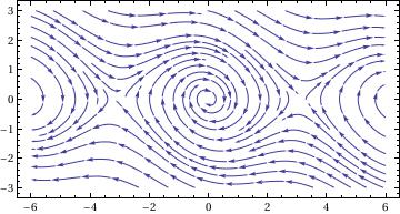
Pendulum numerical simulation
portrait =
StreamPlot[{fx[x, y], fy[x, y]}, {x, -6, 6}, {y, -3, 3},
AspectRatio -> Automatic]
solution =
Function[point, Function @@ {t, ({x[t], y[t]} /.
NDSolve[{x'[t] == fx[x[t], y[t]], y'[t] == fy[x[t], y[t]],
Thred[{x[time], y[time]} == point]}, {x, y}, {t, time,
time + 40}])[[1]]}]
Function[point, Function @@ {t, ({x[t], y[t]} /.
NDSolve[{Derivative[1][x][t] == fx[x[t], y[t]],
Derivative[1][y][t] == fy[x[t], y[t]],
Thred[{x[time], y[time]} == point]}, {x, y}, {t, time, time + 40}])[[1]]}]
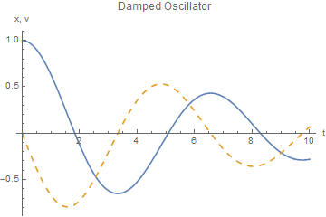
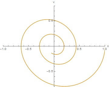
sol1 contains the two interpolating functions (Mathematica uses cubic splines) that represent x(t) and v(t). We can evaluate them or plot
them. For example, the values at t = 3 are
PlotStyle -> {Dashing[{}], Dashing[{0.02, 0.02}]}]
ysol1[t_] := Last[sol1]
sol1 contains the two interpolating functions (Mathematica uses cubic splines) that represent x(t) and v(t). We can evaluate them or plot
them. For example, the values at t = 3 are
PlotStyle -> {Dashing[{}], Dashing[{0.02, 0.02}]}]
ysol1[t_] := Last[sol1]
xsol1 and ysol1.
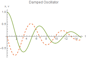
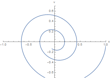
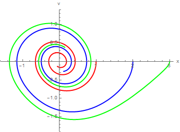
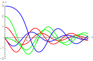
Now we turn to plotting solutions of the pendulum equation subject to distinct initial conditions. Actually, we define three solutions:
sol3 = ans[0.25, 1, 3, 0, 15]
PlotRange -> {{-1.6, 3.1}, {-1.9, 1.4}}, AxesLabel -> {"x", "v"}, PlotStyle -> {{Thick, Red}, {Thick, Blue}, {Thick, Green}}]
PlotRange -> {-2, 3}, PlotStyle -> {{Thick, Red}, {Thick, Blue}, {Thick, Green}}]
Return to Mathematica page
Return to the main page (APMA0340)
Return to the Part 1 Matrix Algebra
Return to the Part 2 Linear Systems of Ordinary Differential Equations
Return to the Part 3 Non-linear Systems of Ordinary Differential Equations
Return to the Part 4 Numerical Methods
Return to the Part 5 Fourier Series
Return to the Part 6 Partial Differential Equations
Return to the Part 7 Special Functions