Return to computing page for the first course APMA0330
Return to computing page for the second course APMA0340
Return to Mathematica tutorial for the first course APMA0330
Return to Mathematica tutorial for the second course APMA0340
Return to the main page for the first course APMA0330
Return to the main page for the second course APMA0340
Return to Part I of the course APMA0340
Introduction to Linear Algebra with Mathematica
Eigenvalues (translated from German, meaning "proper values") are a special set of scalars associated with every square matrix that are sometimes also known as characteristic roots, characteristic values, or proper values.
Each eigenvalue is paired with a corresponding set of so-called eigenvectors.
The determination of the eigenvalues and eigenvectors of a system is extremely important in physics and engineering, where it arises in such common applications as stability analysis, the physics of rotating bodies, and small oscillations of vibrating systems, to name only a few.
We do not discuss computational aspects of eigenvalues/eigenvectors
determination---there are lots of algorithms, and computer codes for doing it, symbolically (precisely) and approximately, for general matrices and special classes of matrices. It should be emphasized that finding eigenvalues involves asking for the determinant of an n × n matrix with entries polynomials, which is slow. Another problem arises when we need to determine roots of corresponding characteristic polynomial.
If A is a square n × n matrix with real entries and v is an \( n \times 1 \)
column vector, then the product w = Av is defined and is another \( n \times 1 \)
column vector. It does not matter whether v is real vector v ∈ ℝn or complex v ∈ ℂn.
Therefore, any square matrix with real entries (we mostly deal with
real matrices) can be considered as a linear operator or transformation A : v ↦ w = Av, acting either in ℝn or ℂn. Of course, one can use any Euclidean space not necessarily ℝn or ℂn.
Although a transformation v
↦ Av may move vectors
in a variety of directions, it often happen that we are looking for
such exceptional vectors on which action of A is just multiplication by a constant. Such a linear transformation is usually referred to as the spectral representation of the operator A.
It is important in many applications to determine nontrivial (nonzero) column vectors v such
that Av is in the same
direction as v, which we denote as
λv. Such special vectors are called eigenvectors of
A that are always exist for any
square matrix A. The eigenvalue λ tells whether the exceptional vector v is stretched or shrunk or reversed or left
unchanged.
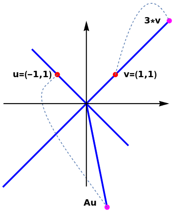
Example 1A:
Let us consider the following matrix and two vectors:
As shown by the plot, v is an eigenvector, but vector u is not an eigenvector of matrix A given that no such constant
exists to map u ↦ A u.
Example 1B:
As another example, we can consider a stochastic matrix that describes the transitions of a Markov chain. Each of its entries is a nonnegative real number representing a probability (in every column, the sum of entries is 1). It is also called a probability matrix, transition matrix, substitution matrix, or Markov matrix.
with respect to the standard basis of ℝ². Here v = [x, y]T is an arbitrary column-vector from ℝ².
In particular, for the vector uk whose coordinates are two consecutive Fibonacci numbers [Fk, Fk-1]T, we have that
Thus, we can produce a vector whose coordinates are two consecutive Fibonacci numbers by applying L many times to the vector u1 with coordinates [F1, F0]T = [1, 0]T:
has a nontrivial solution v (meaning it is not identically zero), then the vector v is called an eigenvector, corresponding to λ,
which is called the associated eigenvalue. The set of all eigenvalues is called the spectrum of matrix A.
There are two pathological matrices that we will avoid in our
exposition: they are the zero matrix 0 (all entries of which
are zeroes) and
the identity
matrix that is denoted by I. Every nonzero vector is an
eigenvector of these two matrices, corresponding to a single
eigenvalue λ = 0 and λ = 1, respectively.
Theorem 1:
If A is an n×n triangular matrix (upper triangular, lower triangular, or diagonal). then the eigenvalues of A are the entries on the main diagonal of A.
Example 3:
We consider the following 5×5 lower triangular matrix
The trace of matrix A is zero as well as its determinant. So its characteristic polynomial is
CharacteristicPolynomial[A, lambda]
-4 lambda + 5 lambda^3 - lambda^5
Note that Mathematica evaluates the characteristic polynomial as det(A - λI), which has the opposite sign to our standard definition.
We can calculate it by evaluating the determinant:
Expand[Det[x*IdentityMatrix[5] - A]]
4 x - 5 x^3 + x^5
■
A number λ can be eigenvalue for a square matrix A only when the determinant of the matrix corresponding to the system \( \lambda \,{\bf v} - {\bf A}\, {\bf v} = {\bf 0} \) vanishes,
namely, \( \det \left( \lambda\, {\bf I} - {\bf A} \right) =0 ,\) where I is the identity matrix.
If A is a square matrix, the determinant \( \chi (\lambda ) = \det \left( \lambda\, {\bf I} - {\bf A} \right) . \) is called the characteristic polynomial and we denote it by χ(λ).
Samuelson's formula allows the characteristic polynomial to be computed recursively without divisions.
Theorem 2:
A scalar (real or complex) is an eigenvalue of a square matrix A if and only if it is a root of characteristic polynomial:
This determinant
is called the characteristic polynomial and we denote it by \( \chi (\lambda ) = \det \left( \lambda\, {\bf I} - {\bf A} \right) . \) Every square matrix has an eigenvalue and corresponding eigenvectors.
Therefore, eigenvalues are the nulls of the characteristic polynomial and they
are the roots of the equation
\( \chi (\lambda ) = 0. \)
The characteristic polynomial is always a polynomial of degree n, where
n is the dimension of the square matrix A. Its
coefficients can be expressed through eigenvalues:
where \( \mbox{tr} {\bf A} = a_{11} + a_{22} + \cdots + a_{nn} = \lambda_1 + \lambda_2 + \cdots + \lambda_n \) is the trace of the matrix A, that is, the sum of its diagonal elements,
which is equal to the sum of all eigenvalues (including their
multiplicities). This is true for arbitrary matrices.
The set of all eigenvalues is called
the spectrum
of the matrix A.
Theorem 3:
A square matrix A is invertible if and only if λ = 0 is not an eigenvalue of A.
Theorem 4:
For any polynomial p(s), if λ is an eigenvalue of a matrix A, and v is a corresponding eigenvector, then p(λ) is an eigenvalue of p(A) and v is a corresponding eigenvector.
Theorem 5:
If λ1, λ2, … , λr are distinct eigenvalues of a square matrix A, and is v1, v2, … , vr are corresponding eigenvectors, then { v1, v2, … , vr } is a linearly independent set.
A defective matrix is a square matrix that does not have a complete basis of eigenvectors.
Mathematica has some special commands (Eigensystem,
Eigenvalues, Eigenvectors, and CharacteristicPolynomial)
to deal with eigenvalues and eigenvectors for square matrices. We show how to
use them in a sequence of examples.
The main command that deals with an eigenvalues problem is
Eigensystem[B], which gives a list {values, vectors} of the
eigenvalues and eigenvectors of the square matrix B.
Out[5]= {lambda -> -I, lambda -> I} (* I is the imaginary unit *)
Mathematica has three different characters to represent the
imaginary unit: I and two others are also used in Wolfram
language when entered into a worksheet with commands \[ImaginaryI] or \[ImaginaryJ], provide outputs 𝕚 or 𝕛, respectively.
To find an eigenvector corresponding to the eigenvalue λ = j, we need to solve the system of equations
Since this quadratic equation \( \det\left( \lambda{\bf I} - {\bf A} \right) = \lambda \left( \lambda -5 \right) = 0 \) has two real roots λ = 0 and λ = 5, we know that these numbers are eigenvalues of matrix A.
Now we use Mathematica; in the following,
the [[1]] indicates the first part of the
expression, which can also be indicated with Part[expression, 1]. In
this case it is negligible because the result is only one part.
v1 = NullSpace[sys[lambda1]][[1]]
{1, 2}
v2 = NullSpace[sys[lambda2]]
{-2, 1}
To check eigenvalues, we type
A.v2==lambda2*v2
True
This can be obtained manually as follows:
A = {{1, 2}, {2, 4}}
Out[1]= {{1, 2}, {2, 4}}
sys[lambda_] = lambda*IdentityMatrix[2]-A
Out[2]= {{-1 + lambda, -2}, {-2, -4 + lambda}}
p[lambda_] =Det[sys[lambda]]
Out[3]= -5 lambda + lambda^2
To find the roots of the characteristic equation (eigenvalues of the matrix
A):
Solve[p[lambda]==0]
Out[4]= {{lambda -> 0}, {lambda -> 5}}
To capture the eigenvalues:
{lambda1,lambda2} = x/.Solve[p[x]==0]
Out[5]= {0, 5}
To show the basis of the null space of the matrix A:
Therefore, we know that the matrix A has one double
eigenvalue λ = 1, and one simple eigenvalue
λ = 0 (which indicates that
matrix A is singular). Next, we find the corresponding
eigenvectors
Eigenvectors[A]
Out[3]= {{1, 0, 0}, {0, 0, 0}, {-1, 1, 0}}
So Mathematica provides us only one eigenvector \( \xi = \left[ 1,0,0 \right] \)
corresponding to the eigenvalue λ = 1 (therefore, A is defective)
and one eigenvector v = <-1,1,0> corresponding
eigenvalue λ = 0. To check this, we introduce the matrix
B1:
B1 = IdentityMatrix[3] - A
Eigenvalues[B1]
Out[5]= {1, 0, 0}
which means that B1 has one simple eigenvalue \( \lambda = 1 \) and one
double eigenvalue \( \lambda =0. \) Then we check that \( \xi \) is an eigenvector
of the matrix A:
B1.{1, 0, 0}
Out[6]= {0, 0, 0}
Then we check that v is the eigenvector corresponding to \( \lambda = 0: \)
A.{-1, 1, 0}
Out[7]= {0, 0, 0}
To find the generalized eigenvector corresponding to \( \lambda = 1, \) we
use the following Mathematica command
LinearSolve[B1, {1, 0, 0}]
Out[8]= {0, -1, -1}
This gives us another generalized eigenvector \( \xi_2 = \left[ 0,-1,-1 \right] \)
corresponding to the eigenvalue \( \lambda = 1 \) (which you can multiply by
any constant). To check it, we calculate:
B1.B1.{0, 1, 1}
Out[9]= {0, 0, 0}
but the first power of B1 does not annihilate it:
B1.{0, 1, 1}
out[10]= {-1, 0, 0}
■
The characteristic polynomial can be found either with
Mathematica's command
CharacteristicPolynomial or multiplying (λ - λk)m for each eigenvalue λk of multiplicity m, when eigenvalues are available.Remember that for odd dimensions, Mathematica's command
CharacteristicPolynomial provides negative value because it is based on the formula det(A - λI) rather than Eq.\eqref{EqEigen.2}.
This means that two equations do not define any constraint on the coordinates of the eigenvector. In other words, all three equations are equivalent and you can take any of them to define a relation between its coordinates.
Therefore, the coordinates of the eigenvectors corresponding to the double eigenvalue λ = 1 are related via the identity
So there are two linearly independent eigenvectors corresponding to the eigenvalue λ = 1; they are [−2, 3, 0]T and [7, 0, 6]T.
■
Return to Mathematica page
Return to the main page (APMA0340)
Return to the Part 1 Matrix Algebra
Return to the Part 2 Linear Systems of Ordinary Differential Equations
Return to the Part 3 Non-linear Systems of Ordinary Differential Equations
Return to the Part 4 Numerical Methods
Return to the Part 5 Fourier Series
Return to the Part 6 Partial Differential Equations
Return to the Part 7 Special Functions