Preface
Since the
Hermite polynomials and Hermite functions are eigenfunctions of corresponding singular Sturm--Liouvivve problems for a second order differential operator, they can be used for expansion of functions into series with respect to these eigenfunctions.
The
Hermite polynomials , conventionally denoted by
H n (
x ) were introduced in 1859 by
Pafnuty Chebyshev . Later, in 1864 they were studied by the French mathematician
Charles Hermite (1822--1901).
Any polynomial (a Hermite polynomial is a particular case) is unbounded on the real axis ℝ = (−∞, ∞), so it does not belong to the Hilbert space 𝔏²(ℝ) of square integrable functions. It turns out that the Hermite polynomials belong to another Hilvert space
𝔏²(ℝ, e −x² ) and also the space of tempered distributions, 𝒮'(ℝ). Fortunately, Hermite polynomials can be used for expansions of tempered distributions into Fourier--hermite series.
The Hermite polynomials \( H_n (x) \) can be defined
"explicitly" as
\begin{equation} \label{EqHermite.1}
H_n (x) = n! \, \sum_{k=0}^{\left\lfloor n/2 \right\rfloor} \frac{(-1)^k}{k! \left( n-2k \right)!} \left( 2x \right)^{n-2k} , \qquad n=0,1,2,\ldots .
\end{equation}
Mathematica has a build-in command for evaluation of the Hermite polynomial:
HermiteH[n, x] .
Since these polynomials contain either even powers of
x or odd powers of
x , depending on the parity of index
n , they possess a
symmetry relation:
\[
H_n (-x) = (-1)^n \,H_n (x) , \qquad n=0,1,2,\ldots .
\]
Hermite polynomials are eigenfunctions of the singular Sturm--Liouville problem for the Hermite differential equation on the infinite interval (−∞, ∞):
\[
y'' -2x\,y' + \lambda\,y =0 , \qquad \mbox{or} \qquad \frac{{\text d}}{{\text d}x} \left( e^{-x^2} \, \frac{{\text d}y}{{\text d}x} \right) + \lambda e^{-x^2}\, y =0, \qquad \lambda = 2n , \quad n\in \mathbb{N} = \{ 0, 1, 2, \ldots \} ,
\]
subject to the condition that its solutions grow at infinity no faster than a polynomial. So
H n (
x )
corresponds to eigenvalue λ
n = 2
n , with
n being a positive integer.
Hermite polynomials can be defined also via
Rodrigues formula
\[
H_n (x) = \frac{\sqrt{\pi}}{2} \left( -1 \right)^n e^{x^2} \frac{{\text d}^{n+1}}{{\text d} x^{n+1}} \mbox{erf}(x) , \qquad \mbox{erf}(x) = \frac{2}{\sqrt{\pi}} \int_0^x e^{-t^2} {\text d}t .
\]
Since the leading coefficient in the Hermite polynomial
H n (
x ) = 2
n x n + ··· grows exponentially. It is convenient to consider similar polynomials but with leading coefficient to be 1.
There exists another sequence {
He n (
x )} of classical orthogonal polynomial called
Chebyshev--Hermite polynomials that are defined explicitly:
\begin{equation} \label{EqHermite.2}
He_n (x) = n! \, \sum_{k=0}^{\left\lfloor n/2 \right\rfloor} \frac{(-1)^k}{2^k \,k! \left( n-2k \right)!} \,x^{n-2k} , \qquad n=0,1,2,\ldots .
\end{equation}
These polynomials are eigenfunctions of the following singular Sturm--Liouville problem
\[
y'' -x\,y' + \lambda\,y =0, \qquad \lambda = n \in \mathbb{N}.
\]
One can define the (normalized) Hermite functions :
\begin{equation} \label{EqHermite.3}
\psi_n (x) = \left( 2^n n! \,\sqrt{\pi} \right)^{-1/2} e^{-x^2 /2} \,H_n (x) = (-1)^n \left( 2^n n! \,\sqrt{\pi} \right)^{-1/2} e^{x^2 /2} \,\frac{{\text d}^n}{{\text d} x^n} \left( e^{-x^2} \right) \qquad n=0,1,2,\ldots
\end{equation}
that form a complete orthonormal basis in 𝔏²(− ∞, ∞). Their Fourier transforms are
\[
\psi_n^F (\xi ) = \hat{\psi}_n (\xi ) = 𝔉_{x\to\xi}\left[ \psi_n (x) \right] (\xi ) = \mbox{P.V.} \int_{-\infty}^{\infty} e^{{\bf j}x\xi} \psi_n (x)\,{\text d}x = {\bf j}^n \sqrt{2\pi}\,\psi_n (\xi ) , \qquad {\bf j}^2 = -1.
\]
Assuming[t > 0,
Integrate[
Exp[I*x*t]*HermiteH[8, x]*Exp[-x^2/2], {x, -Infinity, Infinity}]]
6 E^(-(t^2/2)) Sqrt[
2 \[Pi]] (105 - 840 t^2 + 840 t^4 - 224 t^6 + 16 t^8)
The Hermite functions ψ
n (
x ) is the eigenfunction of the harmnic oscillator:
\[
\left( -\frac{{\text d}^2}{{\text d} x^2} + x^2 \right) \psi_n (x) = \left( 2n+1 \right) \psi_n (x) , \qquad n=0,1,2,\ldots .
\]
There exists another sequence of functions {
h n (
x ) }
n≥0 , called
Chebyshev--Hermite functions that can be defined by the
Rodrigues formula :
\[
h_n (x) = (-1)^n \left( \sqrt{2\pi}\, n! \right)^{-1/2} e^{x^2 /4} \frac{{\text d}^n}{{\text d} x^n} \left( e^{- x^2 /2} \right)
, \qquad n=0,1,2,\ldots .
\]
They are eigenfunction of the harmnic oscillator:
\[
\left( -\frac{{\text d}^2}{{\text d} x^2} + \frac{x^2}{4} \right) h_n (x) = \frac{2n+1}{2}\, h_n (x) , \qquad n=0,1,2,\ldots .
\]
h[n_, x_] = (-1)^n *(Sqrt[2*Pi]*Factorial[n])^(-1/2) *Exp[x^2 /4] *
D[Exp[-x^2 /2], {x, n}];
-(15/2)
Let us consider a set of real-values functions for which the integral (in Lebesque sense)
\[
\left\langle\, f, f \,\right\rangle_w = \| f \|^2 = \int_{-\infty}^{+\infty} \left\vert f(x) \right\vert^2 e^{-x^2} {\text d}x < \infty
\]
is finite, where
w =
e −x² is the weight function. We denote this set as 𝔏²(ℝ,
e −x² ) because its
norm \( \| \cdot \| \) depends on the weight function. With respect to this norm, 𝔏²(ℝ,
e −x² ) becomes
complete . Upon introducing the inner product
\[
\langle f\,\vert\, g \rangle_w = \langle f,g \rangle_w = \int_{-\infty}^{\infty} f(x)\,g(x)e^{−x^2} \,{\text d}x , \qquad w(x) = e^{-x^2} ,
\]
the space 𝔏²(ℝ,
e −x² ) of square
Lebesque integrable functions becomes a
Hilbert space .
The Hermite polynomials are orthogonal with respect to this inner product:
\begin{equation} \label{EqHermite.4}
\langle H_m (x), H_n (x) \rangle = \int_{-\infty}^{\infty} e^{-x^2} H_m (x)\,H_n (x) \,{\text d} x = \begin{cases}
2^n n! \,\sqrt{\pi} , & \quad \mbox{if $n=m$}, \\
0 , & \quad \mbox{if $n\ne m$}. \end{cases}
\end{equation}
Similarly, we introduce the Hilbert space 𝔏²(ℝ, e −x²/2 ) of square Lebesque integrable functions that is equiped with the inner product
\[
\langle f\,\vert\, g \rangle_w = \langle f,g \rangle_w = \int_{-\infty}^{\infty} f(x)\,g(x)e^{−x^2 /2} \,{\text d}x , \qquad w(x) = e^{-x^2 /2} .
\]
Then with respect to this inner product, the Chebyshev--Hermite polynomials become orthogonal:
\begin{equation} \label{EqHermite.5}
\langle He_m (x), He_n (x) \rangle = \int_{-\infty}^{\infty} e^{-x^2 /2} He_m (x)\,He_n (x) \,{\text d} x = \begin{cases}
n!\,\sqrt{2\pi} , & \quad \mbox{if $n=m$}, \\
0 , & \quad \mbox{if $n\ne m$}. \end{cases}
\end{equation}
In the Hilbert space 𝔏²(ℝ, dx ) = 𝔏²(ℝ) of square Lebesque integrable functions, both the
Hermite functions and the Chebushev--Hermite functions are orthonormal with respect to standard inner product:
\[
\int_{-\infty}^{\infty} \psi_n (x) \,\psi_m (x) \,{\text d} x = \delta_{n,m} = \begin{cases}
1 , & \quad \mbox{if $n=m$}, \\
0 , & \quad \mbox{if $n\ne m$}; \end{cases}
\qquad
\mbox{and} \qquad
\int_{-\infty}^{\infty} h_n (x) \,h_m (x) \,{\text d} x = \delta_{n,m} = \begin{cases}
1 , & \quad \mbox{if $n=m$}, \\
0 , & \quad \mbox{if $n\ne m$}. \end{cases}
\]
Hermite functions can be efficiently computed using a three-term recursion relation from two starting values:
\[
\psi_{n+1} (x) = \sqrt{\frac{2}{n+1}} \,x\,\psi_n (x) - \sqrt{\frac{n}{n+1}}\,\psi_{n-1} (x) , \qquad \psi_0 (x) = \pi^{-1/4} e^{-x^2 /2} , \quad \psi_1 (x) = \pi^{-1/4} \sqrt{2}\,x \,e^{-x^2 /2} .
\]
Similarly,
\[
x\,h_n (x) = \sqrt{n+1}\, h_{n+1} (x) + \sqrt{n}\, h_{n-1} (x) , \qquad n=1,2,\ldots .
\]
Since the sequence of Hermite polynomials and Chebyshev--Hermite polynomials form an orthogonal basis of the Hilbert space of functions 𝔏² with weight function \( e^{-x^2} \quad \mbox{or} \quad e^{-x^2 /2} , \) respectively, a square integrable function with such weight, f ∈𝔏²(ℝ, w ), can be expanded into the
Hermite series :
\begin{equation} \label{EqHermite.7}
f (x) = \sum_{n\ge 0} a_n H_n (x) , \qquad a_n = \frac{1}{2^n n! \,\sqrt{\pi}}\, \int_{-\infty}^{\infty} f(x)\, e^{-x^2} \,H_n (x) \,{\text d} x, \qquad n\in \mathbb{N} .
\end{equation}
So its coefficients are ratios:
\[
a_n = \frac{\langle f, H_n \rangle}{\langle H_n , H_n \rangle} = \frac{\langle f, H_n \rangle}{\| H_n \|^2_w} = \frac{1}{n!\,2^n \sqrt{\pi}} \int_{-\infty}^{+\infty} f(t) \,e^{-t^2} H_n (t)\,{\text d}t , \qquad n=0,1,2,\ldots .
\]
Similarly, for f ∈ 𝔏²(ℝ, e −x²/2 ), we have
\begin{equation} \label{EqHermite.6}
f (x) = \sum_{n\ge 0} b_n He_n (x) , \qquad b_n = \frac{1}{n! \,\sqrt{2\pi}}\, \int_{-\infty}^{\infty} f(x)\, e^{-x^2/2} \,He_n (x) \,{\text d} x, \qquad n\in \mathbb{N} .
\end{equation}
From these formulas, we get for f ∈ 𝔏²(ℝ, e −x² ) the Bessel inequality
\[
\sum_{n\ge 0} \frac{\langle \, f(x), H_n (x) \,\rangle^2}{\| H_n (x) \|^2} = \sum_{n\ge 0} \left( \int_{\mathbb{R}} f(t) \,e^{-t^2} H_n (t)\,{\text d}t \right)^2 \le \| f \|^2_w = \int_{-\infty}^{\infty} \left\vert f(x) \right\vert^2 e^{-x^2} {\text d}x .
\]
This series converges in 𝔏p for \( p \in \left( \frac{4}{3} , 4 \right) . \)
Theorem (
Parseval ):
Let
f : (−∞, ∞) → ℝ belongs to the
Hilbert space f ∈ 𝔏²(ℝ,
e −x² ). Then
Parseval's identity holds
\[
\| f(x) \|^2 = \int_{-\infty}^{\infty} \left\vert f(x) \right\vert^2 e^{-x^2} {\text d}x = \sum_{n\ge 0} a_n^2 \| H_n (x) \|^2 = \sqrt{\pi} \sum_{n\ge 0} a_n^2 2^n n! .
\]
Similarly, for
f ∈ 𝔏²(ℝ,
e −x²/2 ), we have
\[
\| f(x) \|^2 = \int_{-\infty}^{\infty} \left\vert f(x) \right\vert^2 e^{-x^2 /2} {\text d}x = \sum_{n\ge 0} b_n^2 \| He_n (x) \|^2 = \sqrt{2\pi} \sum_{n\ge 0} b_n^2 n! .
\]
A function f (x )∈𝔏²(ℝ, dx )
can be expanded over Hermite functions as well (which equivalent to Eq.\eqref{EqHermite.7})
\begin{equation} \label{EqHermite.9}
f(x) = \sum_{n\ge 0} c_n \psi_n (x) , \qquad c_n = \int_{\mathbb{R}} f(x)\,\psi_n (x)\,{\text d}x , \quad n=0,1,2,\ldots .
\end{equation}
A function f ∈ 𝔏²(ℝ) can be also expanded into Fourier--Hermite series with respect to Chebyshev--Hermite functions:
\begin{equation} \label{EqHermite.10}
f(x) = \sum_{n\ge 0} d_n h_n (x) , \qquad d_n = \int_{\mathbb{R}} f(x)\,h_n (x)\,{\text d}x , \quad n=0,1,2,\ldots .
\end{equation}
The series \eqref{EqHermite.10} or \eqref{EqHermite.9}, known as Fourier--Hermite series , converges in 𝔏² sense; however, its pointwise convergence is a very delicated matter.
Theorem (
Parseval ):
Let
f : (−∞, ∞) → ℝ belongs to the
Hilbert space f ∈ 𝔏²(ℝ). Then
Parseval's identities hold
\[
\| f(x) \|^2 = \int_{-\infty}^{\infty} \left\vert f(x) \right\vert^2 {\text d}x = \sum_{n\ge 0} c_n^2 = \sum_{n\ge 0} d_n^2 .
\]
Theorem 3 (Hill--Hermite): x -axis |Im(x )| < w .
When the function
f (
x ) decays only algebraically with |
x |, the convergence of the Hermite series is extremely slow, and thousands of terms may be necessary to obtain an accurate answer.
Theorem 4 (Askey--Wainger): \( S_N [f](x) = \sum_{n=0}^N c_n \psi_n (x) \) of the Fourier--Hermite series \eqref{EqHermite.7} converges to f in the 𝔏p norm if and only if 4/3 < p < 4.
This statement was proved in American Journal of Mathematics ,1965, Vol. 87, pp.695--708.
Theorem 5 (Hermite Truncation Error): for
f (
x ) ∈ 𝔏²(−∞, ∞), we have
\[
\left\vert f(x) - \sum_{n=0}^N c_n \psi_n (x) \right\vert \le 0.816 \, \sum_{n\ge N+1} \left\vert c_n \right\vert .
\]
because
\(
\left\vert \psi_n (x) \right\vert \le 0.816 . \)
Boyd’s book contains a thorough discussion of numerical use of Hermite functions. The rate of convergence of a Hermiteseries depends upon the analytical properties of the solution. In general, both the rateat which the function decays along the real x -axis and also the location of singularities of f (x ) in the complex x -plane affect the asymptotic behavior of the Hermitecoefficients.
We illustrate Hermite series expansions in the following examples. Let us start with a simple monoid function---a power function that can be expanded into finite sum of Hermite's polynomials
\[
x^n = \frac{n!}{2^n} \,\sum_{k= 0}^{\left\lfloor n/2 \right\rfloor} \frac{1}{k! \,(n-2k)!} \, H_{n-2k} (x) = n! \sum_{k= 0}^{\left\lfloor n/2 \right\rfloor} \frac{1}{k! \,2^k \,(n-2k)!} \, He_{n-2k} (x) , \qquad n \in \mathbb{Z}_{+} .
\]
Example 1: Polynomial expansions
Example 1:
We demonstrate the Hermite expansion for the following polynomial \( p(x) = 1 + x + 3 x^2 + 7 x^3 . \) First, we determine its Hermite coefficients and then expand p(x) into Hermite series.
p[x_] = 1 + x + 3 x^2 + 7 x^3
Out[1]= {5/2, 23/4, 3/4, 7/8}
coeffs.Table[HermiteH[n, x], {n, 0, 3}] // Expand
Out[2]= 1 + x + 3 x^2 + 7 x^3
For polynomials, you don't need to do any integrals to find the
expansion. Take a polynomial p and a list basis containing the basis
functions. Then define a function that takes these two, identifies the
variable x, and solves for the coefficients in basis that make the two
polynomials equal in terms of their CoefficientLists .
expandPoly[p_, basis_, x_] :=
expandPoly[1 + x + 3 x^2 + 7 x^3, HermiteH[Range[4] - 1, x], x]
Out[4]= {5/2, 23/4, 3/4, 7/8}
If you already know that you're only interested in a basis of HermiteH, you could incorporate that into the function and do away with the specification of the variable basis as follows:
expandPoly[p_, x_] := # /.
expandPoly[1 + x + 3 x^2 + 7 x^3, x]
Out[6]= {5/2, 23/4, 3/4, 7/8}
a quick change of basis function for polynomials.
hermiteIP[f_, g_, x_] := With[{coeff = CoefficientList[f g, x]},
hermiteExpand[poly_, var_] /; PolynomialQ[poly, var] :=
I used H[n, x] as a place holder for HermiteH[n, x].
hermiteExpand[(1 + x)^5, x]
Out[9]= 39/4 H[0, x] + 95/8 H[1, x] + 25/4 H[2, x] + 15/8 H[3, x] +
5/16 H[4, x] + 1/32 H[5, x]
hermiteExpand[(1 + x)^5, x] /. H -> HermiteH
Out[10]= 39/4 H[0, x] + 95/8 H[1, x] + 25/4 H[2, x] + 15/8 H[3, x] +
5/16 H[4, x] + 1/32 H[5, x]
% // Factor
Out[11]= 1/32 (312 H[0, x] + 380 H[1, x] + 200 H[2, x] + 60 H[3, x] +
10 H[4, x] + H[5, x])
Whenever I want to convert some polynomial expressed with respect to a certain basis in terms of another polynomial basis, my go-to algorithm is Salzer's algorithm. It's rather fast, since it relies only on recurrences. Here's a specialization of that algorithm for the case of monomial-Hermite conversion:
Herbert E. Salzer, A recurrence scheme for converting from one
orthogonal expansion into another. Communications of the ACM, CACM Homepage archive, 1973,
Volume 16, Issue 11, Nov. 1973. https://doi.org/10.1145/35561
Pages 705-707 .
H.E. Salzer, Orthogonal Polynomials Arising in the Numerical Evaluation of Inverse Laplace Transform s, Mathematics of Computation, 1955, Vol. 9, 164-177 (1955)
C.P. Jeffreson, E.-P. Chow, Least squares coefficients for a quadrature formula for Laplace transform inversion, Journal of Computational and Applied Mathematic, 1978, Vol. 4, Issue 1, pp. 53-58. doi: 10.1016/0771-050x(78)90020-7
poly = 1 - x + 2 x^2 - 5 x^4;
c = CoefficientList[poly, x];
n = Length[c] - 1; Remove[a];
a[0, 2] = c[[n - 1]] + c[[n + 1]]/2;
a[1, 2] = c[[n]]; a[2, 2] = c[[n + 1]]/2;
Do[
   a[0, k + 1] = c[[n - k]] + a[1, k]/2;
   a[1, k + 1] = a[0, k] + a[2, k]/2;
   Do[
      a[m, k + 1] = (a[m + 1, k] + a[m - 1, k])/2,
      {m, 2, k - 1}];
   a[k, k + 1] = a[k - 1, k]/2;
   a[k + 1, k + 1] = a[k, k]/2,
   {k, 2, n - 1}];

ccof = Table[a[m, n], {m, 0, n}]
   {1/8, -1, -3/2, 0, -5/8}
monomialToHermite[cofs_?VectorQ] := Module[{n = Length[cofs] - 1, a},
The algorithm as I presented it here uses an implicit two-dimensional array, a, to clearly show off the recurrence. The algorithm can be easily rewritten so that it uses only a pair or so of one-dimensional arrays, but I'll leave out that version for now.
Here's a test of Salzer's method:
monomialToHermite[{1, 1, 3, 7}]
Out[13]= {5/2, 23/4, 3/4, 7/8}
{1, 1, 3, 7}.x^Range[0, 3] == {5/2, 23/4, 3/4, 7/8}.HermiteH[Range[0, 3], x] // Expand
Out[14]= True
CoefficientList[(1 + x)^5, x] // monomialToHermite
Out[15]= {39/4, 95/8, 25/4, 15/8, 5/16, 1/32}
%.HermiteH[Range[0, 5], x] == (1 + x)^5 // Expand
Out[16]= True
As another variation, here's another method based on repeated greedy division:
Reap[Fold[Block[{q, r}, {q, r} = PolynomialQuotientRemainder[#1, #2, x];
Out[18]= {3/2, 5/4, 1/4, 1/8}
Check:
%.HermiteH[Range[0, 3], x] == x^3 + x^2 + x + 1 // Expand
Out[19]= True
Example 1A: Power functions, an even integer
Example 1A: p ∈ℕ, we consider the power function
\[
x_{+}^p = \begin{cases}
x^p , & \ \mbox{ for} \quad x \ge 0, \\
0, & \ \mbox{ for} \quad x \le 0.
\end{cases}
\]
This function does not belong to Hilbert space 𝔏²(−∞, ∞), but it belongs to 𝔏²(ℝ,
e −x² ) and 𝔏²(ℝ,
e −x²/2 ).
Expanding this function into Hermite series, we get
\[
x_{+}^p = \sum_{n\ge 0} a_{p,n} H_n (x) = \sum_{n\ge 0} b_{p,n} He_n (x) ,
\]
where
\[
a_{p,n} = \frac{1}{\| H_n \|^2} \left\langle x_{+}^p , H_n (x) \right\rangle = \frac{1}{2^n n!\,\sqrt{\pi}} \int_0^{\infty} x^p H_n (x) \, e^{-x^2} {\text d} x , \qquad n=0,1,2,\ldots ,
\]
\[
b_{p,n} = \frac{1}{\| He_n \|^2} \left\langle x_{+}^p , He_n (x) \right\rangle = \frac{1}{n!\,\sqrt{2\pi}} \int_0^{\infty} x^p He_n (x) \, e^{-x^2 /2} {\text d} x , \qquad n=0,1,2,\ldots ,
\]
Assuming
p = 2
m ,
m ∈ℕ, we obtain
\[
x_{+}^{2m} = \sum_{n\ge 0} a_{2n} H_{2n} (x) = \sum_{n\ge 0} b_{2n} He_{2n} (x) ,
\]
where
\begin{align*}
a_{2n} &= \frac{1}{2^{2n} (2n)! \,\sqrt{\pi}} \int_0^{\infty} x^{2m} e^{-x^2} H_{2n} (x) \,{\text d} x ,
\\
b_{2n} &= \frac{1}{(2n)! \,\sqrt{2\pi}} \int_0^{\infty} x^{2m} e^{-x^2 /2} He_{2n} (x) \,{\text d} x .
\end{align*}
Using Rodrigues formulae
\begin{align*}
H_{2n} (x) &= (-1)^{2n} e^{x^2} \frac{{\text d}^{2n}}{{\text d} x^{2n}} \, e^{-x^2} ,
\\
He_{2n} (x) &= (-1)^{2n} e^{x^2 /2} \frac{{\text d}^{2n}}{{\text d} x^{2n}} \, e^{-x^2/2} ,
\end{align*}
we get the values of coefficients
\begin{align*}
a_{2n} &= \frac{1}{2^{2n} (2n)! \,\sqrt{\pi}} \int_0^{\infty} x^{2m} \frac{{\text d}^{2n}}{{\text d} x^{2n}} \,e^{-x^2} {\text d} x ,
\\
b_{2n} &= \frac{1}{(2n)! \,\sqrt{2\pi}} \int_0^{\infty} x^{2m} \frac{{\text d}^{2n}}{{\text d} x^{2n}} \,e^{-x^2 /2} {\text d} x .
\end{align*}
Using integration by parts, we derive the formula:
\begin{align*}
\int_0^{\infty} x^{2m} \frac{{\text d}^{2n}}{{\text d} x^{2n}} \,e^{-x^2} {\text d} x &= \frac{(2m)!}{(2m-2n)!} \int_0^{\infty} x^{2m-2n} e^{-x^2} {\text d} x ,
\\
\int_0^{\infty} x^{2m} \frac{{\text d}^{2n}}{{\text d} x^{2n}} \,e^{-x^2 /2} {\text d} x &=
\end{align*}
So we continue:
\begin{align*}
a_{2n} &= \frac{1}{2^{2n} (2n)! \,\sqrt{\pi}} \cdot \frac{(2m)!}{(2m-2n)!} \int_0^{\infty} x^{2m-2n} e^{-x^2} {\text d} x ,
\\
b_{2n} &= \frac{1}{(2n)! \,\sqrt{2\pi}} \cdot
\end{align*}
Remembering the definition of the gamma function
\[
\Gamma (\nu ) = \int_0^{\infty} e^{-t} t^{\nu -1} {\text d} t , \qquad \Re\nu > 0,
\]
we simplify the formulas
\begin{align*}
a_{2n} &= \frac{1}{2^{2n} (2n)! \,\sqrt{\pi}} \cdot \frac{(2m)!}{(2m-2n)!} \cdot \Gamma \left( m-n + \frac{1}{2} \right) ,
\\
b_{2n} &= \frac{1}{(2n)! \,\sqrt{2\pi}} \cdot
\end{align*}
Using the formula for half argument of gamma-function
\[
\Gamma \left( m - n + \frac{1}{2} \right) = \sqrt{\pi} \cdot \frac{(2m-2n)!\, 2^{2n}}{2^{2m} (m-n)!} ,
\]
we simplify coeffiocients further
\begin{align*}
a_{2n} &= \frac{(2m)!}{2^{2m} (2n)!\,(m-n)!} ,
\\
b_{2n} &=
\end{align*}
This allows us to derive the following expressions for Hermite expansions
\[
x^{2m}_{+} = \frac{(2m)!}{4^m} \sum_{n= 0}^m \frac{H_{2n} (x)}{(2n)! \,(m-n)!}
\]
and
\[
x^{2m}_{+} = \sum_{n= 0}^m
\]
Example 1B: Power functions, an odd integer
Example 1B: p ∈ℕ, we consider the power function
\[
x_{+}^p = \begin{cases}
x^p , & \ \mbox{ for} \quad x \ge 0, \\
0, & \ \mbox{ for} \quad x \le 0.
\end{cases}
\]
This function does not belong to Hilbert space 𝔏²(−∞, ∞), but it belongs to 𝔏²(ℝ,
e −x² ) and 𝔏²(ℝ,
e −x²/2 ).
Expanding this function into Hermite series, we get
\[
x_{+}^p = \sum_{n\ge 0} a_{p,n} H_n (x) = \sum_{n\ge 0} b_{p,n} He_n (x) ,
\]
where
\[
a_{p,n} = \frac{1}{\| H_n \|^2} \left\langle x_{+}^p , H_n (x) \right\rangle = \frac{1}{2^n n!\,\sqrt{\pi}} \int_0^{\infty} x^p H_n (x) \, e^{-x^2} {\text d} x , \qquad n=0,1,2,\ldots ,
\]
\[
b_{p,n} = \frac{1}{\| He_n \|^2} \left\langle x_{+}^p , He_n (x) \right\rangle = \frac{1}{n!\,\sqrt{2\pi}} \int_0^{\infty} x^p He_n (x) \, e^{-x^2 /2} {\text d} x , \qquad n=0,1,2,\ldots ,
\]
Assuming
p = 2
m +1,
m ∈ℕ, we obtain
\[
x_{+}^{2m+1} = \sum_{n\ge 0} a_{2n+1} H_{2n+1} (x) = \sum_{n\ge 0} b_{2n+1} He_{2n+1} (x) ,
\]
where
\begin{align*}
a_{2n+1} &= \frac{1}{2^{2n+1} (2n+1)! \,\sqrt{\pi}} \int_0^{\infty} x^{2m+1} e^{-x^2} H_{2n+1} (x) \,{\text d} x ,
\\
b_{2n+1} &= \frac{1}{(2n+1)! \,\sqrt{2\pi}} \int_0^{\infty} x^{2m+1} e^{-x^2 /2} He_{2n+1} (x) \,{\text d} x .
\end{align*}
Using Rodrigues formulae
\begin{align*}
H_{2n+1} (x) &= (-1)^{2n+1} e^{x^2} \frac{{\text d}^{2n+1}}{{\text d} x^{2n+1}} \, e^{-x^2} ,
\\
He_{2n+1} (x) &= (-1)^{2n+1} e^{x^2 /2} \frac{{\text d}^{2n+1}}{{\text d} x^{2n+1}} \, e^{-x^2/2} ,
\end{align*}
we get the values of coefficients
\begin{align*}
a_{2n+1} &= \frac{1}{2^{2n+1} (2n)! \,\sqrt{\pi}} \int_0^{\infty} x^{2m} \frac{{\text d}^{2n+1}}{{\text d} x^{2n+1}} \,e^{-x^2} {\text d} x ,
\\
b_{2n+1} &= \frac{1}{(2n+1)! \,\sqrt{2\pi}} \int_0^{\infty} x^{2m} \frac{{\text d}^{2n+1}}{{\text d} x^{2n+1}} \,e^{-x^2 /2} {\text d} x .
\end{align*}
Example 2: Exponential functions
Example 2:
\[
e^{ax} = e^{a^2 /4} \sum_{n\ge 0} \frac{a^n}{n! \,2^n} \, H_n (x) , \qquad a\in \mathbb{C}, \quad x\in \mathbb{R} .
\]
From this expansion, we have
\[
e^{2x} = e \sum_{n\ge 0} \frac{1}{n!}\, H_n (x) , \qquad e^{-2x} = e \sum_{n\ge 0} \frac{(-1)^n}{n!}\, H_n (x) .
\]
Similarly, we get
\[
e^{-a^2 x^2} = \sum_{n\ge 0} \frac{(-1)^n a^{2n}}{n! \left( 1 + a^2 \right)^{n + 1/2} 2^{2n}}\, H_{2n} (x) .
\]
Upon integration, we obtain Hermite expansion for the
error function :
\[
\mbox{erf}(x) = \frac{2}{\sqrt{\pi}} \int_0^x e^{-t^2} {\text d}t = \frac{1}{\sqrt{2\pi}} \,\sum_{k\ge 0} \frac{(-1)^k}{k! \left( 2k+1 \right) 2^{3k}}\, H_{2k} (x) .
\]
For hyperbolic functions, we have
\[
\cosh (2x) = e \sum_{k\ge 0} \frac{1}{(2k)!}\, H_{2k} (x) , \qquad \sinh (2x) = e \sum_{k\ge 0} \frac{1}{(2k+1)!} \, H_{2k+1} (x) .
\]
Example 3: Trigonometric functions
Example 3:
\[
e^{z^2} \cos (2xz) = \sum_{k\ge 0} (-1)^k \frac{z^{2k}}{(2k)!} \, H_{2k} (x)
\tag{7.1}
\]
and
\[
e^{z^2} \sin (2xz) = \sum_{k\ge 0} (-1)^k \frac{z^{2k+1}}{(2k+1)!} \, H_{2k+1} (x)
\tag{7.2}
\]
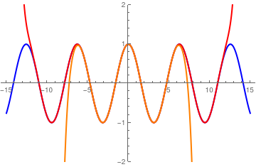
This allows us to expand cos(x ) and sin(x into Hermite series.
\[
\cos (x) = e^{-1/4} \,\sum_{k\ge 0} \frac{(-1)^k}{2^{2k} \, (2k)!} \, H_{2k} (x) .
\tag{7.3}
\]
and
\[
\sin (x) = e^{-1/4} \,\sum_{k\ge 0} \frac{(-1)^k}{2^{2k+1} \, (2k+1)!} \, H_{2k+1} (x) .
\tag{7.4}
\]
Using
Mathematica , we find coefficients in its expansion:
Then we plot its approximation with 10 terms:
Integrate[Cos[x]*HermiteH[6, x]*Exp[-x^2], {x, -Infinity, Infinity}]
In particular,
\[
\cos (2x) = e^{-1} \sum_{k\ge 0} \frac{(-1)^k}{(2k)!}\, H_{2k} (x) .
\]
For sine function, we have
\[
\sin (2kx) = e^{-k^2} \sum_{n\ge 0} (-1)^n \frac{H_{2n+1} (x)}{(2n+1)!} \, k^{2n+1} .
\]
This expansion follows from
\[
\int_{-\infty}^{\infty} \sin (\mu x) \, e^{-x^2 /2} \,H_{2k+1} (x)\,{\text d}x = (-1)^k \sqrt{2\pi} \, e^{-\mu^2 /2} H_{2k+1} (\mu ) .
\]
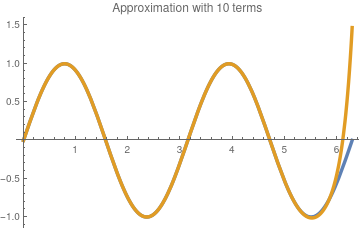
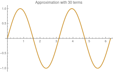
To check the answer, we plot the Hermite approximation with 10 and 30 terms along with function sin[2x ):
sin10[x_] =
Exp[-1]*Sum[(-1)^n *HermiteH[2*n + 1, x]/(2*n + 1)! , {n, 0, 10}];
From the formulas above, we derive the expansion for the
Dirichlet kernel :
\[
\frac{\sin (ts)}{\pi s} = e^{-s^2 /4} \sum_{n\ge 1} (-1)^{n-1} \frac{s^{2n-2}}{\pi \left( 2n-1 \right) !} \, H_{2n-1} (t) , \qquad t\in\mathbb{R} \quad s\in \mathbb{R} \setminus \{ 0 \} .
\]
For the
Fejér kernel , we have
\[
\frac{1 - \cos (st)}{\pi s^2} = \frac{1 -e^{-s^2 /4} }{\pi s^2} + e^{-s^2 /4} \sum_{n\ge 1} (-1)^{n-1} \frac{s^{2n-2}}{4^n \pi \left( 2n \right) !}\, H_{2n} (t)
\]
Example 4: Characteristic functions of symmetric interval
Example 4:
\[
\chi_{[-a,a]}(x) = \begin{cases} 1, & \quad \mbox{for} \quad |x| < a ,
\\
0, & \quad\mbox{for} \quad |x| > a .
\end{cases}
\]
It is assumed that 𝑎 is a positive number. Since the given function is an even function, we get the Hermite expansion:
\[
\chi_{[-a,a]}(x) = \sum_{n\ge 0} c_{2n} H_{2n} (x) , \qquad c_{2n} = \frac{1}{2^{2n} (2n)!\,\sqrt{\pi}} \int_{-a}^a e^{-x^2} \,H_{2n} (x)\,{\text d} x .
\]
Using the recurrence relation
\[
e^{-x^2} \,H_{2n} (x) = - \frac{\text d}{{\text d}x} \left[ e^{-x^2} \,H_{2n-1} (x) \right] , \qquad n\in \mathbb{N} ;
\]
we evaluate coefficients:
\begin{align*}
c_{2n} &= \frac{-1}{\| H_{2n} \|^2} \int_{-a}^a \frac{\text d}{{\text d}x} \left[ e^{-x^2} \,H_{2n-1} (x) \right]
\\
&= \frac{-1}{\| H_{2n} \|^2} \left[ e^{-x^2} \,H_{2n-1} (x) \right]_{x=-a}^{x=a} = \frac{2}{2^{2n} (2n)!\,\sqrt{\pi}}\, e^{-a^2} \, H_{2n-1} (a) .
\end{align*}
In particular,
\begin{align*}
c_0 &= \frac{1}{\sqrt{\pi}} \int_{-a}^a e^{-x^2} {\text d} x = \mbox{erf}(a) ,
\\
c_2 &= \frac{1}{\sqrt{\pi}} \, e^{-a^2} \frac{a}{4} .
\end{align*}
End of Example 4
Example 5: Truncated signum function
Example 5:
\[
\mbox{sign}(x-a) = \begin{cases}
\phantom{-}1 , & \ a < x , \\
-1 , & \ x < a ,
\end{cases}
\]
where 𝑎 is a positive number. We set 𝑎 = 0 for simplicitely, and expand the signum function into Hermite series:
\[
\mbox{sign}(x) = \frac{1}{\sqrt{\pi}} \sum_{k\ge 0} \frac{(-1)^k}{k!\left( 2k+1 \right) k^{2k}}\, H_{2k+1} (x) .
\]
End of Example 5
Example 6: Signum function
Example 6:
\[
\mbox{sign}(x-a) = \begin{cases}
\phantom{-}1 , & \ a < x , \\
-1 , & \ x < a ,
\end{cases}
\]
where 𝑎 is a positive number. We set 𝑎 = 0 for simplicitely, and expand the signum function into Hermite series:
\[
\mbox{sign}(x) = \sum_{k\ge 0} a_{2k+1} H_{2k+1} (x) ,
\]
where
\[
c_{2k+1} = \frac{1}{\| H_{2k+1} \|^2} \int_{-\infty}^{+\infty} e^{-x^2} \mbox{sign}(x)\, H_{2k+1} (x)\,{\text d} x = \frac{2}{2^{2k+1} (2k+1)!\,\sqrt{\pi}} \int_0^{\infty} e^{-x^2} H_{2k+1} (x)\,{\text d} x .
\]
Using the recurrence relation
\[
e^{-x^2} H_{2k+1} (x) = - \frac{\text d}{{\text d}x} \left[ e^{-x^2} H_{2k} (x) \right] ,
\]
we find
\[
c_{2k+1} = \frac{2}{2^{2k+1} (2k+1)!\,\sqrt{\pi}} \, H_{2k} (0)
\]
Taking into accound the formula
\[
H_{2k} (0) = (-1)^k \frac{(2k)!}{k!} ,
\]
we obtain
\[
c_{2k+1} = \frac{(-1)^k}{2^{2k} (2k+1)\,k! \,\sqrt{\pi}}
\]
Then the Hermite expansion of the signum function becomes
\[
\mbox{sign}(x) = \frac{1}{\sqrt{\pi}} \sum_{k\ge 0} \frac{(-1)^k}{2^{2k} (2k+1)\,k!}\, H_{2k+1} (x) .
\]
End of Example 6
Example 7: Sinc function
Example 7:
There are known two
sinc functions : unnormalized (which is used by
Mathematica )
\[
\mbox{sinc}(x) = \frac{\sin x}{x}
\]
and normalized one.
The Hermite series for the normalized
sinc function is
\[
\mbox{sinc}(x) = \frac{\sin \pi x}{\pi x} = \sqrt{\frac{2}{\pi}} \sum_{n\ge 0} \psi_n (x) \,\frac{\sqrt{(2n)!}}{2^n \pi^{1/4}} \,\sum_{k=0}^n \frac{(-1)^k}{(2k)!\left( n-k \right)!} \,2^{3k-1/2} \,\gamma \left( k + \frac{1}{2}, \frac{\pi^2}{2} \right) ,
\]
where ψ
n (
x ) are Hermite functions \eqref{EqHermite.3} and
Gamma[ν, 0, x ] denotes the
lower incomplete gamma function :
\[
\gamma (\nu , x) = \int_0^x t^{\nu -1} e^{-t} {\text d}t .
\]
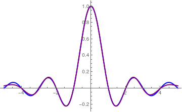
We plot Hermite approximation (in purple) with six terms for the sinc function (in blue):
Plot[{Sinc[Pi*x],
Sum[Sqrt[2/
Pi] Sqrt[(2 n)!]/(2^n Pi^(1/4)) Sum[(-1)^
k/((2 k)! (n - k)!) 2^(3 k - 1/2) Gamma[k + 1/2, 0,
Pi^2/2], {k, 0, n}]* HermiteH[2*n, x]*
Exp[-x^2 /2]/2^n /Pi^(1/4)/Sqrt[(2*n)!], {n, 0, 6}]}, {x, -5, 5},
PlotRange -> All, Evaluated -> True,
PlotStyle -> {{Thick, Blue}, {Thick, Purple}}]
End of Example 7
Example 8: Heaviside function
Example 8: Heaviside function :
\[
H(t) = \begin{cases}
1, & \ \mbox{ for} \quad t > 0 , \\
1/2, & \ \mbox{ for} \quad t = 0, \\
0, & \ \mbox{ for} \quad t < 0.
\end{cases}
\]
Upon expanding it into Hermite series, we obtain
\[
H(t) = \sum_{n\ge 0} c_n H_n (t) ,
\]
where
\[
c_n = \frac{1}{\| H_n \|_w^2} \,\left\langle f(x), H_n (x) \right\rangle = \frac{1}{2^n n! \,\sqrt{\pi}}\, \int_{-\infty}^{\infty} f(x)\, e^{-x^2} \,H_n (x) \,{\text d} x = \frac{n-2}{n \Gamma \left( - \frac{n}{2} \right) n!} \, -@F_1 \left( 1, \frac{1-n}{2}, \frac{1}{2} , 1 \right) .
\]
Mathematica expresses the value of the integral through hypergeometric function:
Integrate[Exp[-x^2]*HermiteH[n, x], {x, 0, Infinity}]
2^n (-2 + n) Sqrt[\[Pi]] Hypergeometric2F1[1, (1 - n)/2, 1/2, 1]
Since the gamma function is unbounded at negative integer values, we get
\[
H(t) = \sum_{k\ge 0} c_{2k+1} H_{2k+1} (t) ,
\]
where
\[
c_{2k+1} = \frac{k-1}{k\, (2k+1)! \Gamma \left( - k - \frac{1}{2} \right)}\,_2F_1 \left( 1, -k , \frac{1}{2} , 1 \right) = \frac{(k-1)\,(-1)^{k+1}}{k\,(2k)!!\,\sqrt{\pi} 2^{k+1}} \,_2F_1 \left( 1, -k , \frac{1}{2} , 1 \right) , \qquad k=0,1,2,\ldots .
\]
End of Example 8
Example 9: Piecewise continuous function
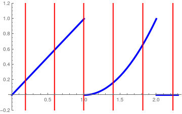
Example 9:
\[
f(x) = \begin{cases}
x, & \ \mbox{ for} \quad 0 < x < 1,
\\
(x-1)^2 , & \ \mbox{ for} \quad 1 < x < 2,
\\
0, & \ \mbox{ otherwise}.
\end{cases}
\]
The corresponding coefficients
c n of the Hermite series
\[
f(x) = \sum_{n\ge 0} c_n H_n (x)
\]
can be determined only numerically
\[
c_n = \frac{1}{\| H_n \|_w^2} \,\left\langle f(x), H_n (x) \right\rangle = \frac{1}{2^n n! \,\sqrt{\pi}}\, \int_{-\infty}^{\infty} f(x)\, e^{-x^2} \,H_n (x) \,{\text d} x = \frac{1}{2^n n! \,\sqrt{\pi}}\left[ \int_0^1 e^{-x^2} \,x \,{\text d} x + \int_1^2 e^{-x^2} \,(x-1)^2 \,{\text d} x \right] .
\]
Mathematica is very helpful wuth their evaluations. Despite that
Mathematica provides analytic formulas,
Integrate[x*Exp[-x^2]*HermiteH[n, x], {x, 1, 2}]
-((Gamma[(1 - n)/2] Hypergeometric1F1[1 + n/2, 5/2, -1])/(
3 Gamma[-n])) - (
2^(-2 + n)
Sqrt[\[Pi]] (-1 + Hypergeometric1F1[1/2 (-1 + n), -(1/2), -1]))/
Gamma[3/2 - n/2]
Integrate[(x - 1)^2*Exp[-x^2]*HermiteH[n, x], {x, 1, 2}]
they are too complicated for numerical utilization. Therefore, we prefer to use numerical integration:
Do[c[n] ==
Pi^(-1/2)/(2^n * n!)*(NIntegrate[
x*Exp[-x^2]*HermiteH[n, x], {x, 0, 1}] +
NIntegrate[(x - 1)^2*Exp[-x^2]*HermiteH[n, x], {x, 1, 2}]), {n,
0, 10}]
Hermite approximation with 30 terms (in red).
Since Hermite and Chebyshev--Hermite polynomials are defined on real axis ℝ, they are unbounded and therefore do not belong to Hilbert space 𝔏²[ℝ]. However, this
Hilbert space contains a subspace of rapidly decreasing functions that is commonly called the
Schwartz space and it is denoted by 𝒮(ℝ) or S(ℝ). Then polynomials can be considered as
functionals on this space.
A smooth function
f : ℝ ↦ ℝ on the Euclidean space ℝ has rapidly decreasing derivatives if the absolute value of the product of any derivative of
f with with any polynomial function is a bounded function. The set of all rapidly decreasing function is denoted by 𝒮(ℝ) or
S (ℝ).
A
tempered distribution on ℝ is a continuous linear functional on the Schwartz space 𝒮(ℝ). The set of tempered
distributions is denoted by 𝒮'(ℝ) or 𝒮*(ℝ) or
S' (ℝ).
A Hermite polynomial or Chebyshev--Hermite polynomial provides an example of tempered distribution, so they belong to 𝒮*(ℝ). On the other hand, every Hermite function or Chebyshev--Hermite function belongs to 𝒮(ℝ).
Every distribution T : 𝒮(ℝ) → ℂ can be written as
\[
T(\phi ) = \langle T, \phi \rangle = \int_{\mathbb{R}} \phi (x)\,T(x)\,{\text d}x
\]
for some function
T (
x ) and any test function ϕ from the Schwartz space.
Theorem 6 (Fourier transform is linear automorphism of Schwartz space):
For
f ∈ 𝔏²(ℝ), its Fourier transform can be expanded as
\begin{equation} \label{EqHermite.8}
f^F (\xi ) = 𝔉_{x\to\xi}\left[ f (x) \right] (\xi ) = \mbox{P.V.} \int_{-\infty}^{\infty} e^{{\bf j}x\xi} f (x)\,{\text d}x = \sqrt{2\pi} \sum_{n\ge 0} {\bf j}^n c_n \psi_n (x) ,
\end{equation}
where coefficients
c n are determined from Eq.\eqref{EqHermite.9}.
Theorem 7:
Every test function ϕ∈𝒮(ℝ) posesses Fourier--Hermite expansion
\[
\phi (x) = \sum_{n\ge 0} c_n \psi_n (x) , \qquad c_n = \langle \phi \,\vert\, \psi_n \rangle ,
\tag{T.1}
\]
or
\[
\phi (x) = \sum_{n\ge 0} d_n h_n (x) , \qquad d_n = \langle \phi \,\vert\, h_n \rangle .
\tag{T.2}
\]
Moreover,
\[
\sum_{n\ge 0} c_n n^p < \infty , \qquad \sum_{n\ge 0} d_n n^p < \infty
\tag{T.3}
\]
for any
p ∈ ℕ = {0, 1, 2, …}. Conversely, if
c n or
d n satisfies (T.3), then the right-hand side of Eq.(T.1) or (T.2) converges to some function ϕ∈𝒮(ℝ).
Similarly, for trmpered distribution
T ∈𝒮'(ℝ), the series
\[
T(x) = \sum_{n\ge 0} c_n \psi_n (x) = \sum_{n\ge 0} d_n h_n (x)
\tag{T.4}
\]
weakly converge and
\[
|c_n | < C\,|n|^k , \qquad |d_n | < C\,|n|^k
\tag{T.5}
\]
for some positive constants
C and
k .
Conversely, if
c n or
d n satisfies (T.5), then the right-hand side of (T.4) converges to some
T ∈𝒮'(ℝ).
The corresponding expansion for Dirac delta function is
\[
\delta (x-a) = \frac{1}{\sqrt{\pi}}\,e^{-(x^2 + a^2 )/2} \, \sum_{n\ge 0} \frac{1}{2^n \, n!}\, H_n (x)\, H_n (a) = \sum_{n\ge 0} \psi_n (x)\,\psi_n (a) .
\]
From this relation, it follows
\[
\sum_{n\in\mathbb{N}} \psi_{2n} (x)\,\psi_{2n} (a) = \frac{1}{2} \left[ \delta (x-a) + \delta (x+a) \right] , \qquad \sum_{n\in\mathbb{N}} \psi_{2n+1} (x)\,\psi_{2n+1} (a) = \frac{1}{2} \left[ \delta (x-a) - \delta (x+a) \right] ,
\]
and
\[
\sum_{n\in\mathbb{N}} \psi_{4n} (x)\,\psi_{4n} (a) = \frac{1}{2\sqrt{2\pi}}\,\cos (ax) + \frac{1}{4} \left[ \delta (x-a) + \delta (x+a) \right] , \qquad \sum_{n\in\mathbb{N}} \psi_{4n+1} (x)\,\psi_{4n+1} (a) = \frac{1}{2\sqrt{2\pi}}\,\sin (ax) + \frac{1}{4} \left[ \delta (x-a) - \delta (x+a) \right] .
\]
Then for even and odd functions, we get
\[
\frac{f(x) + f(-x)}{2} = \sum_{n\in\mathbb{N}} c_{2n} \psi_{2n} (x) = \sum_{n\in\mathbb{N}} c_{4n} \psi_{4n} (x) + \sum_{n\in\mathbb{N}} c_{4n+2} \psi_{4n+2} (x)
\]
and
\[
\frac{f(x) - f(-x)}{2} = \sum_{n\in\mathbb{N}} c_{2n+1} \psi_{2n+1} (x) .
\]
Example 1T: Dirac function
Example 1T:
End of Example 1T
Example 2T: Power functions
Example 2T: p , we consider the general power function
\[
x_{+}^p = \begin{cases}
x^p , & \ \mbox{ for} \quad x \ge 0, \\
0, & \ \mbox{ for} \quad x \le 0.
\end{cases}
\]
Expanding this function into Hermite series, we get
\[
x_{+}^p = \sum_{n\ge 0} a_{p,n} H_n (x) = \sum_{n\ge 0} b_{p,n} He_n (x) = \sum_{n\ge 0} c_{p,n} \psi_n (x) = \sum_{n\ge 0} d_{p,n} h_n (x) ,
\]
where
\[
a_{p,n} = \frac{1}{\| H_n \|^2} \left\langle x_{+}^p , H_n (x) \right\rangle = \frac{1}{2^n n!\,\sqrt{\pi}} \int_0^{\infty} x^p H_n (x) \, e^{-x^2} {\text d} x , \qquad n=0,1,2,\ldots ,
\]
\[
b_{p,n} = \frac{1}{\| He_n \|^2} \left\langle x_{+}^p , He_n (x) \right\rangle = \frac{1}{n!\,\sqrt{2\pi}} \int_0^{\infty} x^p He_n (x) \, e^{-x^2 /2} {\text d} x , \qquad n=0,1,2,\ldots ,
\]
and
\[
c_{p,n} = \left\langle x_{+}^p , \psi_n (x) \right\rangle = \int_0^{\infty} x^p \psi_n (x) \,{\text d} x = \left( 2^n n!\,\sqrt{\pi} \right)^{-1/2} \int_0^{\infty} x^p H_n (x) \, e^{-x^2 /2} {\text d} x , \qquad n=0,1,2,\ldots ;
\]
\[
d_{p,n} = \left\langle x_{+}^p , h_n (x) \right\rangle = \int_0^{\infty} x^p h_n (x) \,{\text d} x = \left( n!\,\sqrt{2\pi} \right)^{-1/2} \int_0^{\infty} x^p H_n (x) \, e^{-x^2 /4} {\text d} x , \qquad n=0,1,2,\ldots .
\]
First, we check some initial values with
Mathematica :
Assuming[p > 0, Integrate[x^p*Exp[-x^2], {x, 0, Infinity}]]
1/2 Gamma[(1 + p)/2]
\[
c_{p,0} = \frac{1}{\sqrt{\pi}}\,\left\langle x_{+}^p , H_0 (x) \right\rangle = \frac{1}{\sqrt{\pi}} \int_0^{\infty} x^p H_0 (x) \,{\text d} x = \frac{1}{2\sqrt{\pi}}\,\Gamma \left( \frac{1+p}{2} \right) .
\]
Assuming[p > 0,
Integrate[x^p*Exp[-x^2]*HermiteH[1, x], {x, 0, Infinity}]]/2/
Sqrt[Pi]
Gamma[1 + p/2]/(2 Sqrt[\[Pi]])
\[
c_{p,1} = \frac{1}{\| H_1 \|^2}\,\left\langle x_{+}^p , H_1 (x) \right\rangle = \frac{1}{2\sqrt{\pi}} \int_0^{\infty} x^p H_1 (x) \,{\text d} x = \frac{1}{2\sqrt{\pi}}\,\Gamma \left( \frac{2+p}{2} \right) .
\]
Assuming[p > 0,
Integrate[x^p*Exp[-x^2]*HermiteH[2, x], {x, 0, Infinity}]]/2^3/
Sqrt[Pi]
(p Gamma[(1 + p)/2])/(8 Sqrt[\[Pi]])
\[
c_{p,2} = \frac{1}{\| H_2 \|^2}\,\left\langle x_{+}^p , H_2 (x) \right\rangle = \frac{1}{2^3 \sqrt{\pi}} \int_0^{\infty} x^p H_2 (x) \,{\text d} x = \frac{p}{8\sqrt{\pi}}\,\Gamma \left( \frac{1+p}{2} \right) .
\]
Assuming[p > 0,
Integrate[x^p*Exp[-x^2]*HermiteH[3, x], {x, 0, Infinity}]]/2^3/6/
Sqrt[Pi]
((-1 + p) p Gamma[p/2])/(48 Sqrt[\[Pi]])
\[
c_{p,3} = \frac{1}{\| H_3 \|^2}\,\left\langle x_{+}^p , H_3 (x) \right\rangle = \frac{1}{2^3 3!\,\sqrt{\pi}} \int_0^{\infty} x^p H_3 (x) \,{\text d} x = \frac{p\left( p-1 \right)}{48\sqrt{\pi}}\,\Gamma \left( \frac{p}{2} \right) = \frac{p-1}{24\sqrt{\pi}}\,\Gamma \left( \frac{p}{2} +1 \right) .
\]
Multipying the recurrence
\[
H_{n+1} (x) = 2x\,H_n (x) - 2n\,H_{n-1} (x)
\]
by
x p and integrating, we obtain
\[
\int_0^{\infty} x^p H_{n+1} (x)\, e^{-x^2} {\text d}x = 2\int_0^{\infty} x^{p+1} H_n (x) \, e^{-x^2} {\text d}x - 2n\,\int_0^{\infty} x^p H_{n-1} (x) \, e^{-x^2} {\text d}x .
\]
This yields the recurrence:
\[
c_{p, n+1} = 2 c_{p+1,n} - 2n\,c_{p, n-1} , \qquad n=1,2,\ldots .
\]
Similarly, multiplying the recurrence
\[
H_{n+1} (x) = 2x\,H_n (x) - H'_{n} (x)
\]
by
x p+1 and integrating, we obtain
End of Example 2T
Example 3T: Signum function
Example 3T:
\[
\mbox{sign}(x-a) = \begin{cases}
\phantom{-}1 , & \ a < x , \\
-1 , & \ x < a ,
\end{cases}
\]
where 𝑎 is a positive number. We set 𝑎 = 0 for simplicitely, and expand the signum function into Hermite series:
\[
\mbox{sign}(x) = \sum_{k\ge 0} a_{2k+1} H_{2k+1} (x) ,
\]
where
\[
c_{2k+1} = \frac{1}{\| H_{2k+1} \|^2} \int_{-\infty}^{+\infty} e^{-x^2} \mbox{sign}(x)\, H_{2k+1} (x)\,{\text d} x = \frac{2}{2^{2k+1} (2k+1)!\,\sqrt{\pi}} \int_0^{\infty} e^{-x^2} H_{2k+1} (x)\,{\text d} x .
\]
Using the recurrence relation
\[
e^{-x^2} H_{2k+1} (x) = - \frac{\text d}{{\text d}x} \left[ e^{-x^2} H_{2k} (x) \right] ,
\]
we find
\[
c_{2k+1} = \frac{2}{2^{2k+1} (2k+1)!\,\sqrt{\pi}} \, H_{2k} (0)
\]
Taking into accound the formula
\[
H_{2k} (0) = (-1)^k \frac{(2n)!}{n!} ,
\]
we obtain
\[
c_{2k+1} = \frac{(-1)^k}{2^{2k} (2k+1)\,k! \,\sqrt{\pi}}
\]
Then the Hermite expansion of the signum function becomes
\[
\mbox{sign}(x) = \frac{1}{\sqrt{\pi}} \sum_{k\ge 0} \frac{(-1)^k}{2^{2k} (2k+1)\,k!}\, H_{2k+1} (x) .
\]
End of Example 5
Signum function is related to the Heaviside function:
\[
H(x) = \frac{1}{2}\left[ \mbox{sign}(x) +1 \right] .
\]
It is known that signum is the Fourier transform of reciprocal of
x :
\[
𝔉_{x\to\xi}\left[ \mbox{P.V.} \frac{1}{x} \right] (\xi ) = \mbox{P.V.} \int_{-\infty}^{+\infty} e^{{\bf j} x\xi} \frac{{\text d}x}{x} = {\bf j} \pi\,\mbox{sign}(\xi ) .
\]
Integrate[Sin[t*x]/x, {x, 0, Infinity}]
(\[Pi] t)/(2 Sqrt[t^2])
Since the Fourier transform of the Heaviside function is known to be
\[
𝔉_{x\to\xi}\left[ H(x) \right] (\xi ) = \int_0^{\infty} e^{{\bf j} x\xi} {\text d}x = \frac{\bf j}{\xi + {\bf j} 0} ,
\]
we can establish the well-known
Lippmann-Schwinger formula:
\[
\frac{1}{x\pm {\bf j}0} = \mbox{P.V.} \frac{1}{x} \mp{\bf j}\,\delta (x) .
\]
Example 4T: Heaviside function
Example 4T: Heaviside function :
\[
H(t) = \begin{cases}
1, & \ \mbox{ for} \quad t > 0 , \\
1/2, & \ \mbox{ for} \quad t = 0, \\
0, & \ \mbox{ for} \quad t < 0.
\end{cases}
\]
Upon expanding it into Hermite series, we obtain
\[
H(t) = \sum_{n\ge 0} c_n H_n (t) ,
\]
where
\[
c_n = \frac{1}{\| H_n \|_w^2} \,\left\langle f(x), H_n (x) \right\rangle = \frac{1}{2^n n! \,\sqrt{\pi}}\, \int_{-\infty}^{\infty} f(x)\, e^{-x^2} \,H_n (x) \,{\text d} x = \frac{n-2}{n \Gamma \left( - \frac{n}{2} \right) n!} \, -@F_1 \left( 1, \frac{1-n}{2}, \frac{1}{2} , 1 \right) .
\]
Mathematica expresses the value of the integral through hypergeometric function:
Integrate[Exp[-x^2]*HermiteH[n, x], {x, 0, Infinity}]
2^n (-2 + n) Sqrt[\[Pi]] Hypergeometric2F1[1, (1 - n)/2, 1/2, 1]
Since the gamma function is unbounded at negative integer values, we get
\[
H(t) = \sum_{k\ge 0} c_{2k+1} H_{2k+1} (t) ,
\]
where
\[
c_{2k+1} = \frac{k-1}{k\, (2k+1)! \Gamma \left( - k - \frac{1}{2} \right)}\,_2F_1 \left( 1, -k , \frac{1}{2} , 1 \right) = \frac{(k-1)\,(-1)^{k+1}}{k\,(2k)!!\,\sqrt{\pi} 2^{k+1}} \,_2F_1 \left( 1, -k , \frac{1}{2} , 1 \right) , \qquad k=0,1,2,\ldots .
\]
References
Boyd, J. P., The Rate of Convergence of Hermite Function Series, Mathematics of Computation, Vol. 35, No. 152, Oct., 1980, American Mathematical Society.
doi: 10.2307/2006396
Davis, Philip,
Interpolation and Approximation,
Dover, 1975,
ISBN: 0-486-62495-1,
LC: QA221.D33
Kagawa, T.: Hermite function expansions of Heaviside function. Journal of Pseudo-Differential Operators and Applications,
2015, 6 , No. 1, pp. 21–32.
Kagawa, T. & Yoshino, K.,
The Hermite expansion of the characteristic functions,
Journal of Pseudo-Differential Operators and Applications,
2017, Vol. 8, No. 2, pp. 255–273.
https://doi.org/10.1007/s11868-017-0188-x
Lewandowska, S. and Mikusiński J., On Hermite expansions of 1/x and 1/|x|, Annales Polonici mathematici, 1974, Vol. 28, pp. 167--172.
Muckenhoupt, B., Mean convergence of Hermite and Laguaerre series , Transactions of the American Mathematical Society , 1970, Volume 147, February, pp. 419--431.
Sadlok, Z. On Hermite expansion of x + p , Annales Polonici mathematici, 1980, 38 , Issue 2, pp. 159--162. doi: 10.4064/ap-38-2-159-162
Sadlok, Z. and Tyc, Z., On Hermite expansions of x k and ln |x |, Annales Polonici mathematici, 1977, Vol. 34, pp. 63--68.
Return to Mathematica page main page (APMA0340) Part 1 Matrix Algebra Part 2 Linear Systems of Ordinary Differential Equations Part 3 Non-linear Systems of Ordinary Differential Equations Part 4 Numerical Methods Part 5 Fourier Series Part 6 Partial Differential EquationsPart 7 Special Functions