Return to computing page for the first course APMA0330
Return to computing page for the second course APMA0340
Return to computing page for the fourth course APMA0360
Return to Mathematica tutorial for the first course APMA0330
Return to Mathematica tutorial for the second course APMA0340
Return to Mathematica tutorial for the fourth course APMA0360
Return to the main page for the first course APMA0330
Return to the main page for the second course APMA0340
Return to Part V of the course APMA0340
Introduction to Linear Algebra with Mathematica
Polynomial solutions of Eq.\eqref{Eqlegendre.1} are conventionally denoted by Pn(x)--- with normalization condition Pn(1) = 1.
Eq.\eqref{Eqlegendre.1} is named after a French mathematician Adrien-Marie Legendre (1752--1833) who introduced these polynomials in 1782.
Legendre's equation comes up in many physical situations involving spherical symmetry.
Legendre polynomials are a special case of Jacobi polynomials, namely, \( \displaystyle \quad P_n (x) = P_n^{(0,0)} (x) , \quad \) where the Jacobi polynomials\( \displaystyle \quad P_n^{(\alpha , \beta )} (x) \quad \) depend on two parameters α, β > −1, and satisfy the Jacobi ODE
\[
\left( 1 - x^2 \right) y'' + \left[ \beta - \alpha - \left( \alpha + \beta + 2 \right) x \right] y' + n \left( n + \alpha + \beta + 1 \right) y = 0 .
\]
where ⌊ · ⌋ is the floor function, and \( \displaystyle \binom{n}{k} = \frac{n!}{k! \,(n-k)!} = \frac{n^{\underline{k}}}{k!} \) is the binomial coefficient.
Let ℭ([−1, 1]) denote all real-valued (or complex-valued, if needed) continuous functions on interval [−1, 1]; and let 𝔄 = {1, P₁(x), P₂(x), …, Pₙ(x), … } be the set of all Legendre polynomials.
By Stone–Weierstrass theorem, algebraic polynomials are uniformly dense in ℭ([−1, 1]). That is, for every f ∈ ℭ([−1, 1]) and every ε > 0, there exists a polynomial q such that
\[
\| f - q \|_{\infty} < \varepsilon.
\]
Thus, polynomials form a dense subspace in ℭ([−1, 1]) with respect to sup norm. Since the orthogonal polynomials (not necessarily Legendre's ones, but arbitrary, including Jacobi's polynomials) span all algebraic polynomials, their linear span is dense in ℭ([−1, 1]) as well. So the set of orthogonal polynomials on [−1, 1] is dense in ℭ([−1, 1]). It is well-known that the set of all continuous functions is dense in the Hilbert space 𝔏²([−1, 1]), therefore, the set of orthogonal polynomials is dense in this Hilbert space.
is called the Dirichlet--Legendre kernel. The partial sum expression can be considered as an integral operator with this kernel,
\[
S_N (f, x) = \int_{-1}^1 K_N (x, t)\,f(t)\, {\text d}t .
\]
To determine the Dirichlet--Legendre kernel, we need the Christoffel–Darboux formula for a sequence of orthogonal polynomials. This formula for Legendre's polynomials was first established by Elwin Bruno Christoffel in 1858; it reads
Step 1 — Start from the three‑term recurrence
Legendre polynomials satisfy:
\[
n+1)P_{n+1}(x)=(2n+1)xP_n(x)-nP_{n-1}(x).
\]
We will use this recurrence twice: once in x, once in y.
Step 2 — Write the recurrence for both variables.
For x:
\[
(2k+1)xP_k(x)=(k+1)P_{k+1}(x)+kP_{k-1}(x).
\]
For y:
\[
(2k+1)yP_k(y)=(k+1)P_{k+1}(y)+kP_{k-1}(y).
\]
Step 3 — Multiply the first by Pk(y) and the second by Pk(x)P_k(x).
So we
multiply the x-equation by Pk(y):
\[
(2k+1)xP_k(x)P_k(y)=(k+1)P_{k+1}(x)P_k(y)+kP_{k-1}(x)P_k(y).
\]
Multiply the y-equation by Pk(x):
\[
(2k+1)yP_k(x)P_k(y)=(k+1)P_{k+1}(y)P_k(x)+kP_{k-1}(y)P_k(x).
\]
Step 4 — Subtract the two equations.
Subtract the second from the first:
Step 5 — Sum from k = 0 to n.
Sum both sides over k = 0, 1, … , n:
Left side:
\[
(x-y)\sum _{k=0}^n(2k+1)P_k(x)P_k(y).
\]
Right side telescopes beautifully:
The terms with k+1 and the terms with k cancel in pairs.
Everything collapses except the top boundary term.
After cancellation, only one term survives:
Step 6 — Divide by x-y.
We obtain:
The final result (Christoffel–Darboux Identity)
This is exactly the identity we wanted.
Example 1:
We start verification with n = 3:
\[
S_3 = 1 + 3\cdot xy + 5\cdot P_2 (x)\,P_2 (y) + 7\cdot P_3 (x)\,P_3 (y) ,
\]
which we plug in into Mathematica:
1 + 3 x y + 5/4 (-1 + 3 x^2) (-1 + 3 y^2) +
7/4 x (-3 + 5 x^2) y (-3 + 5 y^2)
The right-hand side of the Christoffel–Darboux identity becomes
\[
\mbox{rhs}_3 = \frac{4}{x-y} \left[ P_3 (y)\,P_4 (x) - P_3 (x)\,P_4 (y) \right] .
\]
In Mathematica, it reads
We emphasize the main properties of the Dirichlet--Legendre kernels:
Reducing properties for polynomials of degree ≤ N:
\[
\int_{-1}^1 p(t)\, K_N (x,t)\,{\text d}t = p(x) .
\]
Symmetry
\[
K_N (x,t) = K_N (t, x) .
\]
Normalization: the inner product with 1 is
\[
\left\langle 1, K_N (x,\cdot ) \right\rangle = \int_{-1}^1 K_N (x,t)\,{\text d}t = 1 .
\]
because \( \displaystyle \quad \left\langle 1, P_n (\cdot ) \right\rangle = \int_{-1}^1 P_n (x)\,{\text d}t = 0 \quad \) for n = 1, 2, 3, ….
Growth of the Dirichlet--Legendre kernel
\[
\| K_N (x,t) \|_{\infty} \sim N .
\]
𝔏¹ norm grows like lnN.
Not positive.
Localization is weak:
The kernel does not concentrate strongly near t = x. Instead, it has oscillatory tails of size O(1) that decay slowly.
Endpoint behavior is singular:
As x → ±1, the kernel becomes sharply peaked and oscillatory. This reflects the fact that Legendre polynomials have large derivatives near the endpoints---singular points of the Legendre differential equation.
Using Hilb's formula, we have
\[
K_N (x, x) \sim \frac{N}{\pi \sqrt{1 - x^2}} \qquad \mbox{as }\ N \to \infty .
\]
It is convenient to orthonormalize Legendre's polynomials that leads to
Function f(x) must satisfy some stringent conditions for convergence of the Legendre series \eqref{Eqlegendre.4}; among these the continuity of f(x) is neither necessary nor sufficient. The theory of Legendre's series is parallel to that of Fourier series for trigonometric functions.
In case f(x) = xk, where k is a positive integer, it can be seen that f(x) can be represented by a finite series of the polynomials because every monomial xk is a linear combination of the Legendre polynomials:
where the last term of the series is a multiple of P₁(x) = x or P₀(x) = 1, according as k is odd or even. In order to determine coefficients in this finite sum, we have
Therefore,
\[
x^2 = \frac{1}{3} + \frac{2}{3}\, P_2 (x) = \frac{1}{3} + \frac{2}{3}\cdot \frac{1}{2} \left( 3\,x^2 - 1 \right) .
\]
For other first few values of powers, we have
\begin{align*}
x^3 &= \frac{2}{5}\, P_3 (x) +\frac{3}{5}\, P_1 (x) = \frac{2}{5}\cdot \frac{1}{2} \left( 5\,x^3 - 3\,x \right) + \frac{3}{5}\, x ,
\\
x^4 &= \frac{8}{35}\, P_4 (x) + \frac{4}{7}\, P_2 (x) + \frac{1}{5} ,
\\
x^5 &= \frac{8}{63}\, P_5 (x) + \frac{4}{9}\,P_3 (x) + \frac{3}{7}\, P_1 (x) ,
\\
x^6 &= \frac{16}{231}\,P_6 (x) + \frac{24}{77}\,P_4 (x) + \frac{10}{21}\,P_2 (x) + \frac{1}{7} ,
\\
x^7 &= \frac{16}{429}\,P_7 (x) + \frac{8}{39}\,P_5 (x) + \frac{14}{33}\, P_3 (x) + \frac{1}{3}\, x ,
\\
x^8 &= \frac{128}{6435}\,P_8 (x) + \frac{64}{495}\,P_6 (x) + \frac{48}{143}\, P_4 (x) + \frac{40}{99}\, P_2 (x) + \frac{1}{9} .
\end{align*}
We can see that s₄ is a better approximation than the Taylor series in the range [−1, 1].
Actually the distance we minimized involved an integral over the range [−1, 1] so we only expect
that the function s₄(x) is a good approximation in this region. In fact in this range it is a lot closer
on average than the Taylor series. One can calculate that
\[
\| \cos (\pi x) - t_4 (x) \|^2 = \int_{-1}^1 \left( \cos (\pi x) - t_4 (x) \right)^2 {\text d} x = 0.203468 .
\]
NIntegrate[(Cos[Pi*x] - t4[x])^2 , {x, -1, 1}]
0.203468
■
End of Example 2
Theorem 1:
Let {Pₙ(x)}n≥0 be the Legendre polynomials, orthogonal in the Hilbert space of Lebesguesquare integrable functions 𝔏²([−1, 1]) with respect to the weight w(x) = 1. For f ∈ 𝔏²([−1, 1]), define Fourier--Legendre coefficients according to Eq.\eqref{Eqlegendre.5}, and the N-th partial sum
\begin{align} \label{Eqlegendre.6}
S_N (f,x) &= \sum_{n=0}^N P_n (x) \left( n + \frac{1}{2} \right) \int_{-1}^1 f(t)\,P_n (t)\,{\text d}t
\\ \notag
&= \frac{N+1}{2} \int_{-1}^1 \frac{P_{N+1} (x)\,P_N (t) - P_N (x)\, P_{N+1} (t)}{x-t}\,f(t)\,{\text d}t
\\ \notag
&= \int_{-1}^1 f(t)\,K_N (x,t)\,{\text d}t = \left\langle f(\cdot ), K_N (x, \cdot ) \right\rangle .
\end{align}
Then the Fourier-Legendre series \eqref{Eqlegendre.4} converges in mean square sense (in the norm of 𝔏²):
\[
\lim_{N\to\infty} \| f(x) - S_N \|_2 = 0 .
\]
Since the system {Pₙ(x)}n≥0 is orthonormal in the Hilbert space 𝔏²([−1, 1]) , the partial sum SN(f, x) is the orthogonal projection of f onto span{1, P₁, P₂, … , PN} for any N, so
\[
\| f - S_N (f, x) \|_2^2 = \sum_{n=0}^N | c_n |^2
\]
by the Pythagorean theorem in Hilbert space (Bessel's inequality becomes an equality for projections). Letting N → ∞, we obtain the Parseval identity
\[
\| f \|_2^2 = \sum_{n\ge 0} | c_n |^2 ,
\]
and the monotone convergence of the partial sums implies
\[
S_N (f, x) = \sum_{n=0}^N c_n P_n (x) \tof \qquad \mbox{in} \quad 𝔏².
\]
Example 3:
Polynomial expansions is a tool for approximating functions by polynomials. Suppose that we wish
to find a cubic polynomial which approximates cos(πx) well. For instance we may wish to calculate
the value of cos(πx) quickly. It turns out that if the Legendre expansion of cos(πx) is given by
\[
\cos (\pi x) = \sum_{n\ge 0} \left( n + \frac{1}{2} \right) P_n (x) \int_{-1}^1 \cos\left( \pi t \right) P_n (t) \,{\text d} t .
\]
According to Mathematica, its five-term approximation is
\[
T_4 (x) = 1 - \frac{\pi^2 x^2}{2} + \frac{\pi^4 x^4}{24} .
\]
Finally, we plot function cos(πx) and its two approximations with respect to Legendre and Taylor.
Approximate identity:
for any continuous function f,
\[
\sigma_N (x, f) \to f(x) , \qquad \mbox{as } N\to \infty.
\]
Uniform boundedness in 𝔏¹
\[
\left\| K_N^{(1)}(x,\cdot ) \right\|_1 = \int_{-1}^1 K_N^{(1)}(x,t )\,{\text d}t = 1 ,
\]
where norm is evaluated in 𝔏¹([−1, 1]).
Diagonal asymptotics:
Using Hilb's formula and Cesàro summation, we get
\[
K_N^{(1)}(x,x) \sim \frac{2}{\pi \sqrt{1 - x^2}} \qquad \mbox{as } N \to\infty .
\]
Endpoint behavior:
Near x = ±1, the Fejér--Legendre kernel has a boundary layer of width O(1/N²). The kernel remains bounded at the endpoints. It becomes sharply peaked on the scale 1/N².
Smoothness:
The Fejér--Legendre kernel is infinitely differentiable in both variables. Its derivatives satisfy
\[
\left\vert \partial^k_x K_N^{(1)}(x,t) \right\vert \le C_k N^k .
\]
Lemma 1 (Approximate identity property of the Fejér kernels):
Let x ∈ [−1, 1] be fixed. Then for every small positive δ > 0,
\[
\lim_{N\to\infty} \int_{|t-x| > \delta} K_N^{(1)} (x,t)\,{\text d}t = 0.
\]
Equivalently, for each fixed x ∈ [−1, 1], the measures
\[
\mu_A^x (A) = \int_A K_N^{(1)} (x,t)\,{\text d}t
\]
form an approximate identity concentrating at x.
We prove this lemma in two parts:
Interior points x ∈ (−1, 1);
end point x = 1 (and analogously x = −1).
From the Christoffel–Darboux formula and estimate |Pₙ| ≤ 1, we get for x ≠ t that
\begin{align*}
\left\vert K_N (x,t) \right\vert &\le \frac{N+1}{2} \cdot \frac{\left\vert P_{N+1} (x)\, P_N (t) \right\vert + \left\vert P_{N+1} (t)\,P_N (x) \right\vert}{|x-t|}
\\
&\le \frac{N+1}{2} \cdot \frac{1+1}{|x-t|} = \frac{N+1}{|x-t|} .
\end{align*}
For x = t,
\[
K_N (x,x) \le \sum_{n=0}^N \frac{2n+1}{2} = \frac{(N+1)^2}{2} .
\]
Thus. for all x, t ∈ [−1, 1],
\[
\left\vert K_N (x,t) \right\vert \le \min \left\{ \frac{(N+1)^2}{2} , \ \frac{N+1}{|x-t|}\right\} .
\]
For the Fejér--Legendre kernel,
\[
K_N^{91)} (x,t) = \frac{1}{N+1} \sum_{m=0}^N K_m (x,t)
\]
we obtain the crude bound
\[
\left\vert K_N^{(1)} (x,t) \right\vert \le C\,\min \left\{ (N+1)^2 , \ \frac{N+1}{|x-t|} \right\} ,
\]
for some absolute constant C > 0. This is enough for many purposes, but we will sharpen it in the interior via angular parametrization.
Interior pointsx ∈ (−1, 1).
Fix an interior point x ∈ (−1, 1), and write
\[
x = \cos\varphi , \quad t = \cos\theta , \qquad \varphi , \theta \in (0, \pi ) .
\]
We use a standard estimate for Legendre's polynomials in the oscillatory regime:
\[
\left\vert P_n (\cos\theta ) \right\vert \le \frac{C}{\sqrt{n\,\sin\theta}} \qquad \left( C > 0, \ n \ge 1 \right) .
\tag{L.1}
\]
This follows from from the well-known asymptotic expansion
\[
P_n (\cos\theta ) = \sqrt{\frac{2}{\pi n\,\sin\theta}} \,\cos \left( \left( n + \frac{1}{2} \right) \theta - \frac{\pi}{4} \right) + O \left( \frac{1}{n^{3/2}} \right) , \quad \theta \in (0, \pi ), \ n\to \infty ,
\]
uniform in θ ∈ [ε, π − ε], and separate (crude) bound near the endpoints; but for our purposes we treat the above inequality as a known estimate.
In particular, for fixed φ ∈ (0, π),
\[
\left\vert P_n (\cos\varphi )\right\vert \le \frac{C}{\sqrt{n\,\sin\varphi}} \le \frac{C}{\sqrt{n}} .
\]
Thus, there is Cx > 0 depending only on x such that
\[
\left\vert P_n (x) \right\vert \le \frac{C_x}{\sqrt{n+1}} , \qquad n \ge 0 .
\]
Consequently,
\[
\left\vert \hat{P}_n (x) \right\vert = \sqrt{\frac{2n+1}{2}} \left\vert P_n (x) \right\vert \le C_x \sqrt{n+1} \, \frac{1}{\sqrt{n+1}} = C_x ,
\]
so orthonormal Legendre polynomials are uniformly bounded in index n.
Similarly, for variable t = cosθ with θ away from 0 and π, the same estimate holds uniformly on compact subintervals of (−1, 1). This gives better control of KN(x, t) for |θ − φ| not too small.
A Fejér-type bound in the interior
It is a classical result that the orthogonal polynomial setting, for fixed interior x = cosφ, the Fejér kernel behaves like a "bump" of width ∼ 1/(N+1) in the angular variable θ, with height ∼ N+1. To make this precise, one can either:
rely on full Plancherel--Rotach asymptotics and compute the Cesàro averages in the angular variable, or
use estimates on KN plus summation in m to obtain a bound of the form
\[
\left\vert K_N^{(1)} (x, \cos\theta ) \right\vert \le \frac{C_x}{1 + (N+1)^2 (\theta - \varphi )^2} , \quad \theta \in (0, \pi ) .
\]
Rather than fully re-deriving Plancherel--Rotach asymptotics, we state this as a lemma, which is, in essence, the orthogonal-polynomial analogue of the classical Fejér kernel bound on the circle.
Lemma 2 (Fejér kernel bound in the interior):
For each fixed x ∈ (−1, 1), there exists a constant Cx > 0 such that
\[
\left\vert K_N^{(1)} (x, \cos\theta ) \right\vert \le \frac{C_x}{1 + (N+1)^2 (\theta - \varphi )^2} , \qquad \theta \in (0, \pi ), \ x=\cos\varphi ,
\tag{L.2}
\]
for all θ ∈ (0, π), where x = cosφ.
■
We accept Lemma 2 as a classical kernel estimate; it is proved in detail in monographs on orthogonal polynomials (e.g., Szegő, Chapter VII), by combining the Christoffel–Darboux formula, the asymptotics of Pₙ(cosθ), and summation over m ((Fejér averaging).
Fix x ∈ (−1, 1) and δ > 0. We want to show
\[
\int_{|t-x| > \delta} K_N^{(1)} (x,t)\,{\text d}t \ \to \ 0 .
\]
In angular variables, x = cosφ, t = cosθ. The map θ ↦ t = cosθ is smooth and monotone on [0, π]. The condition |t − x| > δ is equivalent to |cosθ − cosφ| > δ, which in turn implies |θ − φ| ≥ cx,δ > 0 (since cosθ is Lipschitz with nonzero derivative at interior points). Formally, there exists η such that
\[
|t-x| > 0 \qquad \Longrightarrow \qquad |\theta - \varphi | > \eta .
\]
The change of variables t = cosθ yields dt = −sinθ dθ, so
\[
\int_{|t-x| > \delta} K_N^{(1)} (x,t)\,{\text d}t = \int_{|\theta - \varphi |> \eta} K_N^{(1)} (x, \cos\theta )\,\sin\theta \,{\text d}\theta .
\]
Using the bound (L.1),
\[
\left\vert \int_{|\theta - \varphi | > \eta} K_N^{(1)} (x, \cos\theta )\,\sin\theta\,{\text d}\theta \right\vert \le \int_{|\theta - \varphi | > \eta} \frac{C_x \,\sin\theta}{1 + (N+1)^2 (\theta - \varphi )^2}\,{\text d}\theta .
\]
For |θ − φ| > η, we have sinθ ≤ 1, so
\[
\le C_x \int_{|\theta - \varphi | > \eta} \frac{{\text d}\theta}{1 + (N+1)^2 (\theta - \varphi )^2} .
\]
Now change variables
\[
u = \left( N+1 \right) \left( \theta - \varphi \right) , \quad {\text d}\theta = \frac{{\text d}u}{N+1} .
\]
Then |θ − φ| > η becomes |u| > (N+1)η. Hence,
\[
\int_{|\theta - \varphi | > \eta} \frac{{\text d}\theta}{1 + (N+1)^2 (\theta - \varphi )^2} = \frac{1}{N+1} \int_{|u| > (N+1)\eta} \frac{{\text d}u}{1 + u^2} .
\]
The integrand 1/(1 + u²) is integrable on ℝ, and its tail integral satisfies
\[
\int_{|u| > (N+1)\eta} \frac{{\text d}u}{1 + u^2} \ \to\ 0 \quad \mbox{as }\ N\to\infty .
\]
Explicitly,
\[
\int_{|\theta - \varphi | > \eta} \frac{{\text d}\theta}{1 + (N+1)^2 (\theta - \varphi )^2} \le \frac{2}{(N+1)\,\eta} .
\]
Thus,
\[
\int_{|\theta - \varphi | > \eta} \frac{{\text d}\theta}{1 + (N+1)^2 (\theta - \varphi )^2}
\le \frac{C'}{(N+1)^2}
\]
some constant C' depending on η.
Consequently,
\[
\int_{|t - x| > \delta} K_N^{(1)} (x,t)\,{\text d}t \ \to \ 0 \quad \mbox{as } N \to \infty
\]
for each fixed interior x. This proves Lemma 1 for x ∈ (−1, 1).
Endpointx = 1.
Now we treat the endpoint x = 1 explicitly, because the angular parametrization degenerates at this point. Let t = cosθ, θ ∈ [0, π]. We fix x = 1.
Let us consider
\[
K_N^{(1)} (1, t) = K_N^{(1)} (1, \cos\theta ).
\]
The corresponding Christoffel–Darboux formula is simplified because Pₙ(1) = 1 for all n:
\begin{align*}
K_m (1, \cos\theta ) &= \sum_{k=0}^m \frac{2k+1}{2} \,P_k (1)\, P_k (\cos\theta ) = \sum_{k=0}^m \frac{2k+1}{2} \,P_k (\cos\theta ) ,
\\
&= \frac{m+1}{2} \cdot \frac{P_{m+1} (\cos\theta ) - P_m (\cos\theta )}{1-\cos\theta} ,
\end{align*}
Thus, we need a bound for this expression.
\[
\left\vert P_{m+1} (\cos\theta ) - P_{m} (\cos\theta ) \right\vert \le \lert\vert P_{m+1} (\cos\theta ) \right\vert + \left\vert P_{m} (\cos\theta ) \right\vert \le 2 .
\]
So
\[
\left\vert K_m (1, \cos\theta ) \right\vert \le \frac{m+1}{2} \cdot \frac{2}{1 - \cos\theta} = \frac{m+1}{1-\cos\theta} .
\]
Hence,
\begin{align*}
\left\vert K_{N}^{(1)} (\cos\theta ) &\le \frac{1}{N+1} \sum_{m=0}^N \frac{m+1}{1-\cos\theta}
\\
&= \frac{1}{1-\cos\theta} \cdot \frac{1}{N+1} \sum_{m=0}^N (m+1)
\\
&= \frac{N+2}{2 \left( 1 - \cos\theta \right)} .
\end{align*}
Using the elementary identity
\[
1 - \cos\theta = 2\,\sin^2 \left( \frac{\theta}{2} \right) ,
\]
we have 1 − cosθ ≥ cθ² for θ ∈ [0, π], with some constant c > 0. Hence,
\[
1 - \cos\theta \ge \frac{2}{\pi^2}\,\theta^2 ,
\]
or
\[
1 - \cos\theta \ge C\,\theta^2 , \qquad 0 \le \theta \le \pi ,
\]
for some absolute constant C. This is our global endpoint bound.
Behavior near the endpoint
We want a better control for small θ, where 1 − cosθ is small. Use Taylor expansion of Pₙ near x = 1.
From the Legendre differential equation
\[
\left( 1 - x^2 \right) P''_n (x) - 2x\,P'_n (x) + n \left( n+1 \right) P_n (x) = 0 ,
\]
we get
\[
\sup_{|x| \le 1} \left\vert P''_n (x) \right\vert \le C\,n^4
\]
for some absolute constant C > 0 (we only need a rough bound). Thus, Taylor's theorem at x = 1 gives
\[
P_n (x) = 1 + P'_n (1) \left( x-1 \right) + \frac{1}{2}\,P''_n (\xi ) \left( x-1 \right)^2 ,
\]
for some ξ between x and 1. Therefore,
\[
P_n (x) = 1 + \frac{n \left( n+1 \right)}{2} \left( x - 1 \right) + R_n (x) ,
\]
where
\[
| R_n (x) | \le \frac{1}{2}\,\sup_{|y|\le 1} \left\vert P''_n (y) \right\vert (x-1)^2 \le C\,n^4 \left( x-1 \right)^2 .
\]
For x = cosθ, θ ∈ [0, 1], say. Then
\[
1 - \cos\theta = \frac{\theta^2}{2} + O\left( \theta^4 \right) ,
\]
and in particular, for sufficiently small θ,
\[
c_1 \theta^2 \le 1 - \cos\theta \le c_2 \theta^2 ,
\]
for some positive constants c₁, c₂. Hence,
\[
P_n (\cos\theta ) = 1 - \frac{n(n+1)}{2}\,(1-\cos\theta ) + O\left( n^4\left( 1- \cos\theta \right)^2 \right)
\]
Now compute the difference:
\[
P_{m+1} (\cos\theta ) - P_m (\cos\theta ) = -(m+1)\,(1-\cos\theta ) + O \left( m^4 (1-\cos\theta )^2 \right) .
\]
Since
\[
(m+1)(m+2) - m(m+1) = (m+1) \left[ (m+2) - m \right] = 2(m+1) ,
\]
Now average over m, we get the value of the Fejér kernel
\begin{align*}
K_N^{(1)} (1, \cos\theta ) &= \frac{1}{N+1} \sum_{m=0}^N K_m (1, \cos\theta )
\\
&= - \frac{1}{2(N+1)} \sum_{m=0}^N \left( m+1 \right)^2 + \cdots .
\end{align*}
The sum of squares is
\[
\sum_{m=0}^N \left( m+1 \right)^2 = \sum_{k=1}^{N+1} k^2 = \frac{(N+1)(N+2)(2N+3)}{6} \sim \frac{(N+1)^3}{3} .
\]
Thus, the main term is of order (N+1)². The error term is
\[
\frac{1}{N+1} \sum_{m=0}^N m^5 \left( 1 - \cos\theta ) \le C\,N^5 \left( 1 - \cos\theta \right) .
\]
So for small θ,
\[
P_n (\cos\theta ) = 1 - \frac{n(n+1)}{4}\,\theta^2 + O \left( n^4 \theta^4 \right) \qquad \theta\to 0 .
\]
Hence, there exists C > 0 such that
\[
\left\vert K_N^{(1)} (1, \cos\theta ) \right\vert \le C\left( (N+1)^2 + N^5 (1-\cos\theta ) \right) , \qquad 0 < \theta \le \pi .
\]
In particular, for θ small enough
\[
N^5 \left( 1 - \cos\theta \right) \le C' \left( N+1 \right)^2 ,
\]
i.e.,
\[
1 - \cos\theta \le \frac{1}{N^5} \quad \iff \quad \theta \le \frac{1}{N^{3/2}} ,
\]
we have
\[
\left\vert K_N^{(1)} (1, \cos\theta ) \right\vert \le \left( N+1 \right)^2 .
\]
Combining with the global bound (L.2), we arrive at
\[
\left\vert K_N^{(1)} (1 - \cos\theta ) \right\vert \lesssim \min \left\{ (N+1)^2 , \ \frac{N+1}{\theta^2} \right\} , \qquad 0 < \theta \le \pi .
\]
This is the endpoint analogue of the Fejér kernel bound in the angular variable.
Endpoint approximate identity
We must show
\[
\int_{|t-1| > \delta} K_N^{(1)} (1, t) \,{\text d}t \ \to \ 0 \quad \mbox{as } N \to \infty ,
\]
for every small δ > 0.
In angular variables t = cosθ with θ ∈ [0, π], the condition |t − 1| > δ is equivalent
\[
1 - \cos\delta > \delta \quad \iff \quad \cos\theta < 1-\delta \quad \iff \quad \theta \ge \theta_0 ,
\]
for some θ₀ = θ₀(δ) ∈ (0, π]. In particular, there exists cδ > 0 such that
\[
\theta \ge \theta_0 \quad \Longrightarrow \quad \theta \ge c_{\delta} > 0 .
\]
Now
\begin{align*}
\int_{|t-1| > \delta} K_N^{(1)} (1, t)\,{\text d}t &= \int_0^{\pi} 1_{1-\cos\theta > \delta} K_N^{(1)} (1, \cos\theta )\,\sin\theta\,{\text d}\theta
\\
&= \int_{\theta \ge \theta_0} K_N^{(1)} (1, \cos\theta )\,\sin\theta\,{\text d}\theta .
\end{align*}
Using global crude bound at the endpoint and sinθ ≤ 1, we get
\[
\left\vert \int_{\theta \ge \theta_0} K_N^{(1)} (1, \cos\theta )\,\sin\theta\,{\text d}\theta \right\vert \le \int_{\theta \ge \theta_0} \left\vert K_N^{(1)} (1, \cos\theta ) \right\vert {\text d}\theta \le C \int_{\theta \ge \theta_0} \frac{N+1}{\theta^2}\,{\text d}\theta .
\]
But θ ≥ θ₀, so
\[
\int_{\theta \ge \theta_0} \frac{N+1}{\theta^2}\,{\text d}\theta = \left( N+1 \right) \left[ -\frac{1}{\theta} \right]_{\theta_0}^{\pi} = \left( N+1 \right) \left( \frac{1}{\theta_0} - \frac{1}{\pi} \right) \sim \frac{N+1}{\theta_0} .
\]
This bound grows with N, so we have to be more careful: the global bound is too crude. Instead, we exploit the fact that the Fejér kernel at x = 1 has total mass 1, and the large values of the kernel are confined to a small neighborhood of size ∼ 1/(N+1). In particular, we have
For θ ≤ α/(N+1), we have \( \displaystyle \quad K_N^{(1)} (1, \cos\theta ) \le (N+1)^2 . \)
For θ ≥ α/(N+1), we have, which is integrable in θ on [α/(N+1), π] with total integral O(1), and moreover that integral tends to 0 as we push the lower limit to a fixed θ₀.
A standard way to make this precise is:
Fix δ > 0, let θ₀ be as above. Choose N large enough so that
\[
\frac{\alpha }{N+1}<\theta _0.
\]
Then
\[
\{ \theta \geq \theta _0\} \subset \left\{ \theta \geq \frac{\alpha }{N+1}\right\} .
\]
Hence,
\[
\int _{\theta \geq \theta _0}|F_N(1,\cos \theta )|\, d\theta \leq \int _{\theta \geq \alpha /(N+1)}\frac{C(N+1)}{\theta ^2}\, d\theta =C(N+1)\left[ \, -\frac{1}{\theta }\right] _{\alpha /(N+1)}^{\pi }=C\left( \frac{N+1}{\alpha /(N+1)}-\frac{N+1}{\pi }\right) =C\left( \frac{(N+1)^2}{\alpha }-\frac{N+1}{\pi }\right) .
\]
This estimate alone still grows like (N+1)², but recall that the total mass of \( \displaystyle \quad K_N^{(1)} (1, \cos\theta )\,\sin\theta\,{\text d}\theta \quad \) is 1:
\[
\int_0^{\pi} K_N^{(1)} (1, \cos\theta )\,\sin\theta\,{\text d}\theta = \int_{-1}^1 K_N^{(1)} (1, t)\,{\text d}t = 1 .
\]
Thus, the contribution from small region θ ≤ α/(N+1), where the Fejér kernel ∼ (N+1)², is of order
\[
\int _0^{\alpha /(N+1)}(N+1)^2\sin \theta \, d\theta \sim (N+1)^2\cdot \frac{\alpha }{N+1}=\alpha (N+1),
\]
which would blow up unless the implicit constants are such that the mass remains 1; in fact, precise asymptotics (coming from Bessel kernels) show that:
the height is ≈ N+1, not (N+1)², in the correct normalization for dt.
Since we have been very crude, a fully rigorous endpoint estimate would require invoking the exact Fejér-type kernel representation in angular variables (similar to the trigonometric case), or a direct appeal to the general theory in Szegő: the Fejér kernel associated with Legendre polynomials is nonnegative, normalized, and forms an approximate identity at every point in [-1,1], including endpoints. That is, Lemma 4.1 holds in full generality, and the endpoint requires no special exception in the abstract theory.
Lemma 2 (Endpoint estimate of the Fejér kernels at x = 1):
Let
\[
K_N^{(1)} (x,t) = \sum_{n=0}^N \left( 1 - \frac{n}{N+1} \right) \left( n + \frac{1}{2} \right) P_n (x)\,P_n (t) , \qquad x,t \in [-1, 1],
\]
be the Fejér--Legendre kernel. Then there exist a positive constant C such that for all integers N ≥ 0 and all θ ∈ (0, π],
Define the partial sum kernel
\[
K_m (x,t) = \sum_{n=0}^m \left( n + \frac{1}{2} \right) P_n (x)\,P_n (t) .
\]
The Christoffel--Darboux formula gives
\[
K_m (x,t) = \frac{m+1}{2}\cdot \frac{P_{m+1}(x)\, P_m (t) - P_m (x)\,P_{m+1} (t)}{x-t} .
\]
At x = 1, since Pm(1) = 1, we have
\begin{equation*}
K_m(1,t)
=
\frac{(m+1)}{2} \cdot \frac{\bigl(P_{m+1}(t)-P_m(t)\bigr)}{1-t}.
\end{equation*}
Hence,
\begin{equation*}
K_N^{(1)} (1,t)
=
\frac{1}{N+1}\sum_{m=0}^N K_m(1,t)
=
\frac{1}{N+1}\sum_{m=0}^N
\frac{(m+1)}{2} \cdot \frac{\bigl(P_{m+1}(t)-P_m(t)\bigr)}{1-t}.
\end{equation*}
In angular variables t = cosθ,
\begin{equation*}
F_N(1,\cos\theta)
=
\frac{1}{N+1}\sum_{m=0}^N
\frac{(m+1)}{2} \cdot \frac{\bigl(P_{m+1}(\cos\theta)-P_m(\cos\theta)\bigr)}
{1-\cos\theta},
\qquad 0<\theta\le\pi.
\end{equation*}
Global crude bound.
Since |Pₙ(cosθ)| ≤ 1 for all n and θ ∈ [0, π],
\[
\bigl|P_{m+1}(\cos\theta)-P_m(\cos\theta)\bigr|\le2,
\]
and therefore
\begin{equation*}
\left\vert K_m(1,\cos\theta) \right\vert
\le
\frac{(m+1)}{1-\cos\theta}.
\end{equation*}
Using
\begin{equation*}
1-\cos\theta
=
2\sin^2\!\left(\frac{\theta}{2}\right)
\ge
\frac{2}{\pi^2}\,\theta^2,
\qquad 0\le\theta\le\pi,
\end{equation*}
we obtain
\begin{equation*}
\left\vert K_m(1,\cos\theta) \right\vert
\;\lesssim\;
\frac{m+1}{\theta^2},
\qquad 0<\theta\le\pi.
\end{equation*}
Averaging in $m$ yields
\[
\left\vert K_N^{(1)}(1,\cos\theta) \right\vert
\le
\frac{1}{N+1}\sum_{m=0}^N |K_m(1,\cos\theta)|
\lesssim
\frac{1}{N+1}\sum_{m=0}^N \frac{m+1}{\theta^2}
\lesssim
\frac{N+1}{\theta^2}.
\tag{L2.1}
\]
Height bound at θ = 0.
At t = 1,
\[
K_N^{(1)}(1,1)
=
\frac{1}{N+1}\sum_{n=0}^N \frac{2n+1}{2}\cdot P_n(1)^2
=
\frac{1}{N+1}\sum_{n=0}^N \frac{2n+1}{2} .
\]
Since
\[
\sum_{n=0}^N (2n+1) = (N+1)^2,
\]
we obtain
\begin{equation*}
K_N^{(1)}(1,1) = N+1.
\end{equation*}
By positivity of the Fejér kernel,
\begin{equation*}
0\le K_N^{(1)} (1,t)\le K_N^{(1)}(1,1)=N+1,
\qquad t\in[-1,1],
\end{equation*}
and thus
\[
\left\vert K_N^{(1)} (1,\cos\theta) \right\vert
\le N+1,
\qquad 0\le\theta\le\pi.
\tag{L2.2}
\]
Fejér--type scaling.
Combining (L2.1) and (L2.2), we get
\begin{equation*}
\left\vert K_N^{(1)} (1,\cos\theta) \right\vert
\;\lesssim\;
\min\!\left\{\,N+1,\ \frac{N+1}{\theta^2}\right\},
\qquad 0<\theta\le\pi.
\end{equation*}
For all θ > 0,
\begin{equation*}
\min\!\left\{1,\ \frac{1}{(N+1)^2\theta^2}\right\}
\;\lesssim\;
\frac{1}{1+(N+1)^2\theta^2}.
\end{equation*}
Multiplying by N+1,
\begin{equation*}
(N+1)\min\!\left\{1,\ \frac{1}{(N+1)^2\theta^2}\right\}
\;\lesssim\;
\frac{N+1}{1+(N+1)^2\theta^2}.
\end{equation*}
Hence, there exists C > 0 such that
\[
\left\vert K_N^{(1)} (1,\cos\theta) \right\vert
\;\le\;
\frac{C\,(N+1)}{1+(N+1)^2\theta^2},
\qquad 0<\theta\le\pi,
\tag{L2.3}
\]
which is exactly the required inequality.
Approximate identity away from θ = 0.
Fix θ₀ > 0. Using Eq.(L2.3), we have
\[
\int_{\theta\ge\theta_0}
\left\vert K_N^{(1)} (1,\cos\theta) \right\vert \sin\theta\,{\text d}\theta
\le
C\int_{\theta_0}^{\pi}
\frac{(N+1)}{1+(N+1)^2\theta^2}\,{\text d}\theta.
\tag{L2.4}
\]
Since
\begin{equation*}
\frac{\text d}{{\text d}\theta}\arctan\bigl((N+1)\theta\bigr)
=
\frac{N+1}{1+(N+1)^2\theta^2},
\end{equation*}
we compute
\begin{equation*}
\int_{\theta_0}^{\pi}
\frac{(N+1)}{1+(N+1)^2\theta^2}\,{\text d}\theta
=
\arctan\bigl((N+1)\pi\bigr)
-
\arctan\bigl((N+1)\theta_0\bigr).
\end{equation*}
Using the asymptotic expansion
\begin{equation*}
\arctan z
=
\frac{\pi}{2}-\frac{1}{z}+O(z^{-3}),
\qquad z\to+\infty,
\end{equation*}
we obtain
\[
\arctan\bigl((N+1)\theta_0\bigr)
=
\frac{1}{N+1}\left(\frac{1}{\theta_0}-\frac{1}{\pi}\right)
+O\!\left((N+1)^{-3}\right)
\longrightarrow 0
\tag{L2.5}
\]
as N → ∞. Combining (L2.4) and (L2.5) yields
the second inequality.
Theorem 2:
For any integrable f ∈ 𝔏¹([−1, 1]), the Legendre series \eqref{Eqlegendre.4} is Cesàro-summable to f(x) at almost every point x ∈ [−1, 1].
This is a special case of general summability results for orthogonal polynomial expansion in Szego's book (§7.3--§7.5).
Stein–Weiss present essentially the same scheme for expansions associated with self-adjoint operators, viewing Fejér operators as positive contractions approximating the identity in 𝔏p, and then invoking Lebesgue differentiation for the boundary behavior. A deep insight is given in articles by Pollard and Muckenhoupt.
So we need to show that
\begin{align*}
\sigma _N \left( f,x\right) &= \frac{1}{N+1}\sum _{k=0}^N S_k (f,x) = \frac{1}{N+1}\sum _{k=0}^N \int_{-1}^1 K_k (x,t)\,f(t)\,{\text d}t
\\
&= \int_{-1}^1 K_N^{(1)} (x,t)\,f(t)\,{\text d}t
\end{align*}
converges to f(x) for almost every x. Here the Dirichlet kernel is
\begin{align*}
K_n (x,t) = \sum_{k=0}^n \hat{P}_k (x)\, \hat{P}_k (t) = \sum_{k=0}^n P_k (x) \left( k + \frac{1}{2} \right) P_k (t)
\\
&= \frac{n+1}{2}\cdot \frac{P_{n+1} (x)\,P_n (t) - P_n (x)\,P_{n+1} (t)}{x-t} , \quad x \ne t .
\end{align*}
The Fejér kernel is
\begin{align*}
K_N^{(1)} (x,t) &= \frac{1}{N+1} \sum_{m=0}^N K_m (x,t)
\\
&= \sum_{n=0}^N \left( 1 - \frac{n}{N+1} \right) \hat{P}_n (x)\,\hat{P}_n (t)
\\
&= \sum_{n=0}^N \left( 1 - \frac{n}{N+1} \right) \left( n + \frac{1}{2} \right) P_n (x)\,P_n (t) .
\end{align*}
We need three properties:
Symmetry and normalization:
\[
K_N^{(1)}(x,t) = K_N^{(1)}(t,x)
\]
by definition (the Legendre polynomials appear in Eq.(4) symmetrically).
Positivity: for all N ∈ ℕ and all x, t ∈ [−1, 1], we have
\[
K_N^{(1)} (x,t) \ge 0 .
\]
Proof: For each index m ≥ 0, let Pm : ℌ → ℌ be the orthogonal projection onto the finite dimensional subspace
\[
V_m = \mbox{span}\left\{ P_0 , P_1 , P_2 , \ldots , P_m \right\} .
\]
Then Pm is self-adjoint and idempotent, and
\[
P_m f = \sum_{n=0}^m \left( \int_{-1}^1 f(t)\,\hat{P}_n (t)\,{\text d}t \right) \hat{P}_n (x) = S_m (f , x) .
\]
Define the Fejér operator
\[
T_N f := \frac{1}{N+1} \sum_{m=0}^N P_m f .
\]
Then σNf = TN. Each Pm is positive in the following sense: if f ≥ 0 almost everywhere, then Pmf ≥ 0 almost everywhere (this can be justified either by an explicit kernel representation, or via spectral theory for self-adjoint projectors on real &Lfr'²; this is standard in the theory of orthogonal expansions). A convex combination of positive operators is positive, so if f ≥ 0, then
\[
\sigma_N (f, x) = T_N f (x) \ge 0 \quad \mbox{a.e. } x.
\]
On the other hand, we have the integral representation
\[
\sigma_N (f, x) = \int_{-1}^1 K_N^{(1)} (x,t)\,f(t)\,{\text d}t .
\]
Fix x₀ ∈ [−1, 1] and N. Suppose that for the sake of contradiction, that there exists a set
\[
E = \left\{ t \in [-1, 1] \ : \ K_N^{(1)} (x,t) < 0 \right\}
\]
with positive measure. Choose f ≥ 0 supported in E, nontrivial. Then
\[
\sigma_N \left( f , x_0 \right) = \int_{-1}^1 K_N^{(1)} (x_0 ,t)\,f(t)\,{\text d}t \le \int_E K_N^{(1)} (x_0 ,t)\,f(t)\,{\text d}t < 0 ,
\]
contradicting positivity of TN. Therefore, the Fejér kernel is positive for almost every t. By continuity in t (as finite sum of continuous functions), we get positivity of the Fejér kernel for all t ∈ [−1, 1]. Since x₀ was arbitrary, the claim follows.
Normalization: For every x ∈ [−1, 1] and every positive integer N, we have
\[
\int_{-1}^1 K_{N}^{(1)} (x,t)\,{\text d}t = 1 \qquad \forall x \in [-1, 1] .
\]
Proof: Since integral over the Legendre polynomial is zero, \( \displaystyle \quad \int_{-1}^1 P_n (x, t)\,{\text d}t = 0 \quad n=1,2,\ldots , \quad \) we get
\begin{align*}
\int_{-1}^1 K_{N}^{(1)} (x,t)\,{\text d}t &= \int_{-1}^1 \sum_{n=0}^N \left( 1 - \frac{n}{N+1} \right) \left( n + \frac{1}{2} \right) P_n (x) \,P_n (t)\,{\text d}t
\\
&= \sum_{n=0}^N \left( 1 - \frac{n}{N+1} \right) \left( n + \frac{1}{2} \right) P_n (x) \,\int_{-1}^1 P_n (t)\,{\text d}t
\\
&= \sum_{n=0}^N \left( 1 - \frac{n}{N+1} \right) \left( n + \frac{1}{2} \right) P_n (x) \,2\,\delta_{n,0}
\\
&= \sum_{n=0}^N \left( 1 - \frac{0}{N+1} \right) \left( 0 + \frac{1}{2} \right) P_0 (x)\,2 = 1 .
\end{align*}
because \( \displaystyle \quad \int_{-1}^1 P_0 (x,t)\,{\text d}t = 2 \quad \) and \( \displaystyle \quad \int_{-1}^1 P_n (x,t)\,{\text d}t = 0 \quad \) for k ≥ 1. Hence
\[
\int_{-1}^1 K_N^{(1)}(x,t)\,{\text d}t = \sum_{k=0}^N \left( 1 - \frac{0}{N+1} \right) \left( 0 + \frac{1}{2} \right) P_0 (x) \cdot 2 = 1
\]
Its 𝔏¹ norm is
\[
\left\| K_N^{(1)}(x,t) \right\|_1 = \int_{-1}^1 K_N^{(1)}(x,t) \,{\text d}t = 1 .
\]
To prove pointwise convergence, we need to establish that the Fejér kernels form an approximate identity for each x. This approach is based on determination of estimates for the Dirichlet and Fejér kernels; these formulas are standard consequences of the Christoffel–Darboux formula and the differential equation for Legendre's polynomials, and are treated in detail in monographs such as Szegő's book.
For x ≠ t, we have
\[
K_N (x,t) = \frac{N+1}{2}\cdot \frac{P_{N+1}(x)\,P_N (t) - P_N (x)\,P_{N+1} (t)}{x-t} .
\]
The Legendre polynomials are bounded |Pₙ(x)| ≤ 1 on interval [−1, 1] and all indices. Hence
\begin{align*}
\left\vert K_N (x,t) \right\vert &\le \frac{N+1}{2}\cdot \frac{|P_{N+1}(x)\,P_N (t)| + |P_N (x)\,P_{N+1} (t)|}{|x-t|}
\\
&\le \frac{N+1}{2}\cdot \frac{1+1}{|x-t|}
\\
&= \frac{N+1}{|x-t|} .
\end{align*}
Therefore,
\[
\left\vert K_N (x,t) \right\vert \le \frac{N+1}{|x-t|} , \qquad x \ne t .
\]
For x = t, one can use the orthonormal expansion:
\begin{align*}
\left\vert K_N (x,x) \right\vert &= \sum_{n=0}^N \hat{P}_n^2 (x) = \sum_{n=0}^N \frac{2N+1}{2} \,P_n^2 (x)
\\
&\le \sum_{n=0}^N \frac{2N+1}{2} = \frac{(N+1)^2}{2} .
\end{align*}
So we have a combined estimate
\[
\left\vert K_N (x,x) \right\vert \le \min \left\{ \frac{(N+1)^2}{2}, \ \frac{N+1}{|x-t|} \right\} .
\]
It follows that
\begin{align*}
\left\vert K_N^{(1)} (x,t) \right\vert &= \frac{1}{N+1} \left\vert \sum_{m=0}^N K_m (x,t) \right\vert
\\
&\le \frac{1}{N+1} \sum_{m=0}^N \min \left\{ \frac{(m+1)^2}{2} , \ \frac{m+1}{|x-t|} \right\} .
\end{align*}
This yields
\[
\left\vert K_N^{(1)} (x,t) \right\vert \min \left\{ (N+1)^2 , \ \frac{N+1}{|x-t|} \right\} .
\]
uniformly in x, t ∈ [−1, 1]. The qualitative picture is
Near the diagonal t = x, the Fejér kernel can be as large as ∼ (N + 1)².
Away from the diagonal, the kernel decays like (N + 1)/|x - t|.
For the endpoint x = 1, one often writes t = cosθ and uses more refined expansions in θ; but the estimate above is enough to capture the approximate identity behavior in 𝔏¹.
We state the approximate identity property precisely. Lemma: Let x ∈ [−1, 1] be fixed. Then for every δ > 0,
\[
\lim_{N\to\infty} \int_{|t-x| > \delta} K_N^{(1)} (x,t)\,{\text d}t = 0.
\]
Sketch of proof: Because \( \displaystyle \quad K_N^{(1)} (x,t) \ge 0 \quad \) and \( \quad \int_{-1}^1 K_N^{(1)} (x,t)\,{\text d}t =1. \quad \) it suffices to show that for each fixed δ > 0,
\[
\sup_{|t-x| > \delta} K_N^{(1)} (x,t) \ \to \ 0 \quad \mbox{as }\ N \to \infty .
\]
That is, the Fejér kernels become uniformly small away from the diagonal. For orthogonal polynomials of the Legendre type on a compact interval such bounds follow from the asymptotic behavior of the Christoffel–Darboux kernel: one has Plancherel--Rotach type asymptotic for Pm, which apply that
\[
K_N (x,t) = O(1) , \quad |t-x| > \delta ,
\]
with the implicit constant depending on δ but not on N. In particular,
\[
K_N (x,t) = \frac{1}{N+1} \sum_{m=0}^N K_m (x, t) = O(1)
\]
for |t − x| ≥ δ. However, the normalization
\[
\int_{-1}^1 K_N (x,t)\,{\text d}t = 1
\]
forces the mass to concentrate near x. Indeed, if a uniform positive proportion of the mass were retained outside |t − x| ≤ δ, then normalization together with the bound \( \displaystyle \quad K_N^{(1)} (x,t) = O(1) \quad \) away from x would contradict the growth \( \quad K_N^{(1)} (x,t) \ \sim \ c(x)\,(N+1) \quad \) on shrinking neighborhoods. A rigorous version of this argument is standard in the theory of orthogonal polynomials: see Szegő's book, Chapter VII, where general conditions are given under which the Cesàro kernels of orthogonal expansions form an approximate identity.
For the purpose of the present theorem we take Lemma as known; it is the Legendre polynomial analogue of the standard fact that the trigonometric Fejér kernel converges weakly to the delta measure and forms an approximate identity.
■
Convergence at Lebesgue points:
Let f ∈ 𝔏¹([−1, 1]). By the Lebesgue differentiation theorem, almost every x ∈ [−1, 1],
\[
\lim_{r\downarrow 0} \int_{x-r}^{x+r} \left\vert f(t) - f(x) \right\vert {\text d}t = 0 .
\]
Such x are called Lebesgue points of f.
Fix Lebesgue point x. We shall show that
\[
\lim_{N\to\infty} \sigma_N (f , x) = f(x) .
\]
Recall
\[
\sigma_N (f, x) = \int_{-1}^1 K_N^{(1)} (x,t) \,f(t)\,{\text d}t .
\]
Using normalization of the Fejér kernel, we rewrite
\[
\sigma_N (f, x) - f(x) = \int_{-1}^1 K_N^{(1)} (x,t) \left[ f(t) - f(x) \right] {\text d}t .
\]
Let ε > 0. Since x is a Lebesgue point, there exists δ > 0 such that
\[
\frac{1}{2\delta} \int_{x-\delta}^{x+\delta} \left\vert f(t) - f(x) \right\vert {\text d}t < \varepsilon .
\]
Split the integral into "near" and "far" part:
\[
\sigma_N (f,x) - f(x) = I_N^{near} + I_N
\]
where
\[
I_N^{near} = \int_{|t-x| \le\delta} K_N^{(1)} (x,t) \left\vert f(t) - f(x) \right\vert {\text d}t .
\]
Near part
We use only positivity and normalization of the kernel near x. Since the
Fejér kernels are nonnegative,
\[
\left\vert I_N^{near} \right\vert \le \int_{|x-t| \le \delta} K_N^{(1)} (x,t) \left\vert f(t) - f(x) \right\vert {\text d}t .
\]
Introduce the probability measure
\[
{\text d}\mu (t) = K_N^{(1)} (x,t) \,{\text d}t \qquad \mbox{on } \ [-1, 1] .
\]
Then
\[
\left\vert I_N^{near} \right\vert \le \int_{|x-t| \le\delta} \left\vert f(t) - f(x) \right\vert {\text d}\mu_n (t) .
\]
However, the restriction of μN to the interval [x − δ, x + δ] is dominated by a probability measure supported there (it is in fact already a sub-probability measure). In particular,
\[
\left\vert I_N^{near} \right\vert \le \sup_{\nu} \int_{x-\delta}^{x+\delta} \left\vert f(t) - f(x) \right\vert {\text d}\nu (t) ,
\]
where ν runs over all probability measures supported in [x − δ, x + δ]. The largest such integral (for absolutely continuous measures) is obtained by the normalized Lebesgue measure, so
\[
\left\vert I_N^{near} \right\vert \le \frac{1}{2\delta} \int_{x-\delta}^{x+\delta} \left\vert f(t) - f(x) \right\vert {\text d}t < \varepsilon .
\]
This estimate is uniform in N. Therefore,
\[
\sup_{N> 0} \left\vert I_N^{near} \right\vert \le \varepsilon .
\]
Far part:
We use the approximate identity property of the Fejér kernels
First treat bounded function f. Suppose f ∈ 𝔏∞([−1, 1]). Then
\[
\left\vert f(t) - f(x) \right\vert \le 2 \, \| f \|_{\infty} ,
\]
and hence
\begin{align*}
\left\vert I_N^{far} \right\vert &\le \int_{|x-t| > \delta} K_N^{(1)} (x,t) \left\vert f(t) - f(x) \right\vert {\text d}t
\\
&\le \| f \|_{\infty} \int_{|x-t| > \delta} K_N^{(1)} (x,t) \,{\text d}t .
\end{align*}
By Lemma,
\[
\int_{|x-t| > \delta} K_N^{(1)} (x,t) \,{\text d}t \ \to \ 0 \quad \mbox{as} \quad N\to\infty .
\]
Therefore,
\[
I_N^{far} \ \to \ 0 \quad \mbox{as} \quad N\to\infty
\]
for bounded functions.
For general f ∈ 𝔏¹, approximate f by bounded functions f(k) (for instance, truncate f at levels ±k). The Fejér operators are bounded on 𝔏¹ (indeed, they are positive, preserve constants, and are contractions on 𝔏²; interpolation gives boundedness on 𝔏p for 1 ≤ p ≤ 2, and density argument extends the pointwise convergence result from bounded f to all f ∈ 𝔏¹). This is standard in the general theory of Fejér/Cesàro summability of orthogonal series and mimics exactly the Fourier series.
Thus, for our fixed Lebesgue point x,
\[
\lim_{N\to\infty} I_N^{far} = 0 .
\]
Conclusion:
Combining the two parts, we have for all ε > 0,
\[
\limsup_{N\to\infty} \left\vert \sigma_N (f, x) - f(x) \right\vert \le \sup_N \left\vert I_N^{near} \right\vert + \limsup_{N\to\infty} \left\vert I_N^{far} \right\vert \le \varepsilon + 0 .
\]
Since ε > 0 was arbitrary, it follows that
\[
\lim_{N\to\infty}\sigma_N (f, x) = f(x) .
\]
This identity holds at each Lebesgue point x of f, and by the Lebesgue differentiation theorem such points form a set of full measure in [−1, 1]. The theorem 2 is proved.
Remarks:
The structure of the Fejér kernel here is exactly parallel to the trigonometric Fejér kernel \( \displaystyle \quad F_n (x) = \frac{1}{n}\,\sum_{k=0}^{n-1} D_k (x) , \quad \) which is nonnegative, normalized, and forms an approximate identity on the circle.
The genuinely nontrivial step is Lemma (approximate identity property), which rests on asymptotics of Christoffel–Darboux kernels and Legendre polynomials. This is treated in detain in Szegő's monograph (chapter VII). In a more general setting (orthogonal polynomials with respect to positive weights on compact intervals), and our Legendre case satisfies all the necessary hypotheses.
No essential modification is needed at the endpoints: the Lebesgue differentiation theorem applies with intervals [1 −r, 1], and the Fejér kernels still form an approximate identity in the appropriate sense. If desired, one may rewrite the kernels near x = 1 in the angular variable t = cosθ to get explicit bounds of the form
\[
K_N^{(1)} (1, \cos\theta ) \le \min \left\{ (N+1)^2 , \ \frac{N+1}{\theta^2} \right\} ,
\]
that makes the concentration near fully explicit.
■
Approximate identity: abstract framework.
We recall the general notion needed for the convergence theorem,
Let (X, μ) be a measure space, here X = [−1, 1] with Lebesgue measure. A family of kernels Kα(x, t) (α is a parameter) is called approximate identity if
Uniform 𝔏¹ bound
\[
\sup_{\alpha} \sup_{x \in [-1,1]} \int_{-1}^1 K_{\alpha} (x, t)\,{\text d}t < \infty .
\]
In our case, positivity + normalization gives this bound with constant 1.
Localization (vanishing tails:
\[
\lim_{\alpha \to \infty} \sup_{x \in [-1,1]} \int_{-1+\delta}^{1-\delta} \left\vert K_{\alpha} (x, t)\right\vert {\text d}t = 0 \qquad \forall \delta > 0 .
\]
Then for any f ∈ 𝔏¹([−1, 1]), the operators
\[
T_{\alpha} f(x) = \int_{-1}^1 f(t)\, K_{\alpha} (x,t)\,{\text d} t
\]
converge to f(x) at every Lebesgue point of f, and hence almost everywhere.
So for almost everywhere convergence, what we must prove is that the Fejér kernels form an approximate identity.
We already have items 1 and 2. The key remaining point is the localization. So we want to show that
\[
\lim_{\alpha \to \infty} \sup_{x \in [-1,1]} \int_{-1+\delta}^{1-\delta} \left\vert K_{N}^{(1)} (x, t)\right\vert {\text d}t = 0 \qquad \forall \delta > 0 .
\]
Intuition tells us that as N grows, the Fejér kernels concentrates more and more near the diagonal t = x with tails that carry vanishing mass.
Interior points x away from endpoints (singular points).
Fix ε > 0. Consider x in a compact subinterval [−1 + &epsilon, 1 − ε]. There we can use Hilb's asymptotics for Legendre polynomials: if x = cosθ, t = cosϕ , then for large n,
\[
P_n (\cos\theta ) \sim \sqrt{\frac{2}{\pi n \sin\theta}}\, \cos \left( \left( n + \frac{1}{2} \right) - \frac{\pi}{4} \right)
\]
and similarly for Pₙ(cosϕ).
Plugging the series expression
\[
K_N^{(1)} (x,t) = \sum_{n=0}^N \left( 1 - \frac{n}{N+1} \right) \left( n + \frac{1}{2} \right) P_n (x)\, P_n (t) ,
\]
we see that for x and t in the interior region and with |x − t| ≥ δ, the phase oscillates with respect to n. The factor 1 −n/(N+1) is a Cesàro wight; standard summation methods (Dirichlet--Abel summation or direct adaption of Fourier--Fejér analysis) show that the sum over n then behaves like a localized bump whose mass concentrates near, and whose integral over |θ − ϕ| ≥ δ tends to zero as N → ∞.
Informally, away from the line t = x, the oscillations in n cancel out, and Cesàro averaging suppresses the cancellations even more strongly. More precisely, one shows that for fixed δ > 0 and ε > 0,
\[
P_n (\cos\theta ) = \sqrt{\frac{\theta}{\sin\theta}} \, J_0 \left( \left( n + \frac{1}{2} \right) \theta \right) + O \left( \frac{1}{n} \right) ,
\]
and hence by positivity and normalization,
\[
\lim_{n \to \infty} \sup_{x \in [-1+\varepsilon , 1-\varepsilon ]} \int_{-1+\delta}^{1-\delta} K_{N}^{(1)} (x, t)\, {\text d}t = 0 \qquad \forall \delta > 0 .
\]
Indeed, for fixed positive δ, there is a constant C(δ) such that
\[
\int_{|t i x| \ge \delta} \left\vert K_N^{(1)} (x,t) \right\vert {\text d}t \le \frac{C(\delta )}{N} \to 0 .
\]
So we have localization uniformly for x away from the endpoints.
Near the endpoints, our previous estimates such as
\[
\left\vert K_N^{(1)} (x,t) \right\vert \le \frac{C}{|x - t|}
\]
do not work because the kernel involves denominators like
\[
\sqrt{1 - x^2}\,\sqrt{1 - t^2} ,
\]
or their angular versions, which behave like 1/(sinθ sinϕ). These estimates are harmless when θ, ϕ are bounded away from 0, π, but they blow up near the endpoints.
Using the Christoffel–Darboux formula, the Fejér kernel can be written as
\[
K_N^{(1)} (x,t) = \frac{1}{N+1} = \sum_{k=0}^N \frac{k+1}{2} \cdot \frac{P_{k+1} (x)\, P_k (t) - P_k (x)\, P_{k+1} (t)}{x-t} .
\]
For x = 1, we have
\[
K_N^{(1)} (1,t) = \frac{1}{N+1} = \sum_{k=0}^N \frac{k+1}{2} \cdot \frac{P_{k+1} (1)\, P_k (t) - P_k (1)\, P_{k+1} (t)}{1-t} .
\]
Since Pₙ(1) = 1 for any nonnegative integer n, we come to the telescopic series
\[
A = \sum_{k=0}^N \left( k+1 \right) P_k (t) - \sum_{k=0}^N \left( k+1 \right) P_{k+1} (t) .
\]
In the second sum, we change the index of summation by putting j = k+1. This yields
\[
\sum_{k=0}^N \left( k+1 \right) P_{k+1} (t) = \sum_{j=1}^{N+1} j\,P_j (t) .
\]
So
\[
A = \sum_{k=0}^N \left( k+1 \right) P_k (t) - \sum_{k=1}^{N+1} k\,P_k (t) = 1 - \left( N+1 \right) P_{N+1} (t) + \sum_{k=1}^N P_k (t) .
\]
Now we show the uniform boundness of the 𝔏¹ norm of the Fejér kernel. Fixing a small positive δ, we split the integral
\[
\int_{-1}^1 \left\vert K_N^{(1)} (1,t) \right\vert {\text d}t = \int_{-1}^{1-\delta} \left\vert K_N^{(1)} (1,t) \right\vert {\text d}t + \int_{1-\delta}^1 \left\vert K_N^{(1)} (1,t) \right\vert {\text d}t .
\]
We need bounds independent of N.For t being fae away from t = 1, |t − 1| ≥ δ, the denominator 1 − t is bounded away from zero: 1 − t ≥ δ. So from the spliting formula, we get
\[
\left\vert K_N^{(1)} (1,t) \right\vert \le \frac{1}{2 \left( N+1 \right) \delta} \left( \left\vert \sum_{k=0}^N P_k (t) \right\vert + \left( N+1 \right) \left\vert P_{N+1} (t) \right\vert \right) .
\]
A single Legendre polynomial is uniform;y bounded:
\[
\left\vert P_{N+1} (t) \right\vert \le C_2 (\delta ) , \quad t \in [-1, 1-\delta ], \quad \forall N .
\]
We use a classical fact about partial sum of Legendre polynomials (both uniform in N for fixed t ∈ [−1, 1 − δ])
\[
\left\vert \sum_{k=0}^N P_k (t) \right\vert \le C_1 (\delta ) , \quad t\in [-1, 1-\delta ], \quad \forall N ,
\]
with some positive constant C₁(δ). (This comes from the generating function for the Legendre polynomials.) This gives a uniform estimate of 𝔏¹ norm doe t away from the endpoint t = 1.
Near t = 1, we set t = cosθ. Then t = 1 corresponds small θ. So on interval [1 − δ, 1] we have θ ∈ [0, θ₀] with θ₀ determined by cosθ₀ = 1 − δ. Then
\[
{\text d}t = -\sin\theta\,{\text d}\theta , \quad 1-t = 1 - \cos\theta \sim \frac{\theta^2}{2} .
\]
The integral becomes
\[
I_N^{\tiny near} = \int_{1-\delta}^1 \left\vert K_{N}^{(1)} (1,t) \right\vert \le {\text d}t = \int_0^{\theta_0} \left\vert K_{N}^{(1)} (1,\cos\theta ) \right\vert \sin\theta\,{\text d}\theta .
\]
Now the telescopic formula in θ-form becomes
\[
K_{N}^{(1)} (1,\cos\theta ) = \frac{1}{2 \left( N+1 \right) \left( 1 - \cos\theta \right)} \left( \sum_{k=0}^N P_k (\cos\theta ) - \left( N+1 \right) P_{N+1} (\cos\theta ) \right) .
\]
Using small angle behavior
\[
1 - \cos\theta \sim \frac{\theta^2}{2} , \qquad \sin\theta \sim \theta ,
\]
the prefactor behaves like
\[
\frac{\sin\theta}{1 - \cos\theta} \sim \frac{\theta}{\theta^2 /2} = \frac{2}{\theta} .
\]
Thus, for small θ, we get
\[
\int_{1-\delta}^1 \left\vert K_{N}^{(1)} (1,\cos\theta ) \right\vert \sin\theta\,{\text d}\theta \le
\]
Now we apply the standard asymptotic input (Hilb type asymptotic):
for each compact θ-interval [0, θ₀] and all N ≥ 1,
\[
\left\vert P_n (\cos\theta ) \right\vert \le C \left( 1 + n\theta \right)^{-1/2} .
\]
Consequently,
\[
\left\vert \sum_{k=0}^N P_k (\cos\theta ) \right\vert \le C\,\min \left\{ N+1 , \frac{1}{\sqrt{\theta}} \right\} .
\]
Accepting these inequalities (they are standard can be derived from Bessel-function approximations), you get
The term with PN+1:
\[
\frac{1}{N+1} \cdot \frac{1}{\theta} \left( N+1 \right) \left\vert P_{N+1} (\cos\theta ) \right\vert \le \frac{C''}{\theta} \left( 1 + N\theta \right)^{-1/2} .
\]
The term with sum of the Legendre polynomials:
\[
\frac{1}{N+1} \cdot \frac{1}{\theta} \left\vert \sum_{k=0}^N P_k (\cos\theta ) \right\vert \le
\]
=================================
Bessel/Mehler--Heine scaling.
Near the endpoints, we use Mehler--Heine type asymptotics. For example, near x = 1, write
\[
x = \cos\frac{u}{N}, \qquad \phi = \cos\frac{v}{N} ,
\]
with u, v of order 1. Then
\[
P_n \left( \cos\frac{u}{N} \right) \to J_0 (u) \qquad \mbox{as } n\to\infty .
\]
Summing with Fejér weights in the Legendre case corresponds, under this scaling to constructing Bessel-type Fejér kernel in the variables u, v
Lebesgue differentiation theorem: for almost every point, the value of an integrable function is the limiting average taken around the point.
Almost everywhere Cesàro convergence of the Legendre series does not imply 𝔏¹-convergence of the Cesàro means. However, they converge in 𝔏² sense but fail to converge in 𝔏¹([−1, 1]) for several reasons. It is known that 𝔏²([−1, 1]) ⊂ 𝔏¹([−1, 1]), and the Fejér kernels are uniformly bounded,
but not uniformly integrable in 𝔏¹.
Example 4:
We consider an integrable, but not a square integrable function
\[
f(x) = \frac{1}{\sqrt{1-x}} .
\]
Its Legendre coefficients are all the same and equal to √(2)
Approximations via Legendre (red) and Taylor (purple).
This picture shows that the Taylor approximation is much better than Legendre's one, which does not approximate function 1/√(1−x).
For clarification, let us consider function g(x) = (1 − x)¼ that belongs to 𝔏²([−1, 1]) and 𝔏¹([−1, 1]). Expanding this function into Legendre series with the aid of Mathematica, we obtain its fourth degree approximation:
\[
s_4 (x) = \frac{1}{3}\,2^{7/4} + \frac{1}{7} \,2^{7/4}\,x + \frac{50}{231}\, 2^{3/4}\,P_2 (x) + \frac{2}{11}\, 2^{3/4}\,P_3 (x) + \frac{234}{1463}\, 2^{3/4}\,P_4 (x) .
\]
Approximations via Legendre (ref) and Taylor (purple).
Since it is not clear which of these approximations (Legendre or Taylor) gives better approximation to function g(x), we estimate the distances in 𝔏² of these approximations:
\[
\left\| (1 - x )^{1/4) - s_4 (x) \right\|^2 = \int_{-1}^1 \left[ (1 - x )^{1/4) - s_4 (x) \right]^2 {\text d} x = 0.0645418 .
\]
These numbers show that Legendre's approximation provides better job compares to Taylor's one.
■
End of Example 4
Theorem 3:
If f ∈ ℭ([−1, 1]) is a continuous function, then its Cesàro means
\[
\sigma_N (f, x) = \sum_{n=0}^N \left( 1 - \frac{n}{N+1} \right) P_n (x) \left( n + \frac{1}{2} \right) \int_{-1}^1 f(t)\,P_n (t)\,{\text d}t \ \to \ f(x)
\]
uniformly on [−1, 1] as N → ∞.
Recall that the Fejér--Legendre kernel is
\[
K_N^{(1)} (x,t) = \frac{1}{N+1} \sum_{k=0}^N K_N (x,t) ,
\]
where the Legendre--Dirichlet kernel is
\[
K_N (x, t) = \sum_{n=0}^N \frac{2n+1}{2} \, P_n (x)\,P_n (t) .
\]
Write
\[
\sigma_N(f;x)-(f,x)
=\int_{-1}^1 \left( f(t)-f(x)\right) K_N^{(1)} (x,t)\,{\text d}t.
\]
For f ∈ ℭ([−1, 1]), fix ε > 0 and choose δ > 0 such that
\[
| f(t) - f(x)| < \varepsilon \quad \mbox{whenever} \quad |t-x| < \delta .
\]
Split the integral:
\[
\sigma_N(f;x)-f(x)
=I_1(x,N)+I_2(x,N),
\]
where
\begin{align*}
I_1(x,N) &= \int_{|t-x|<\delta} (f(t)-f(x))K_N^{(1)}(x,t)\,{\text d}t,
\\
I_2 (x,N) &=\int_{|t-x|\ge\delta} (f(t)-f(x))K_N^{(1)}(x,t)\,{\text d}t.
\end{align*}
For I₁,
\[
\left\vert I_1(x,N)\right\vert
\le \varepsilon \int_{-1}^1 \left\vert K_N^{(1)} (x,t)\right\vert {\text d}t
\le C\varepsilon .
\]
For I₂,
\[
\left\vert I_2(x,N) \right\vert
\le 2\|f\|_\infty
\int_{|t-x|\ge\delta} |K_N^{(1)} (x,t)|\,{\text d}t.
\]
By the approximate identity property, the last integral tends to 0
uniformly in x.
Thus for all sufficiently large N,
\[
\sup_{x\in[-1,1]}|\sigma_N(f;x)-f(x)|
\le C\varepsilon + \varepsilon.
\]
Since ε > 0 is arbitrary, the convergence is uniform.
𝔏²-convergence does not imply pointwise convergence. Extra smoothness of f yields stronger modes of convergence, but the Hilbert-space proof above is purely 𝔏². The pointwise convergence for piecewise continuous functions of bounded variation is presented next.
Theorem 4:
If function f∈ 𝔏([−1, 1]) of bounded variation on [-1,1] (or f satisfies the Dirichlet conditions on the interval [−1, 1]), then its Legendre series converges at every interior point x ∈ (-1,1) to
where coefficients cn are determined according to Eq.\eqref{Eqlegendre.5}.
This theorem was proved in the article by Bojanić and Vuilleumier. Conditions on function f can be reformulated as follows.
Let interior point x ∈ (−1, 1) be fixed. It is assumed that
f has bounded variation on some open interval (x − δ, x + δ) for some δ > 0;
the one-sided limits f(x − 0) and f(x + 0) exist and finite.
We are looking for the classical result: if f is piecewise continuous and of bounded variation on [-1,1], then its Fourier–Legendre series converges at each x to \frac{f(x^+)+f(x^-)}{2}. Below is a clean proof using the Christoffel–Darboux kernel and an approximate identity argument.
\[
K_N(x,t):=\sum _{n=0}^N\frac{2n+1}{2}\, P_n(x)\,P_n(t).
\]
We split the proof into three steps.
Step 1: Christoffel--Darboux and kernel representation.
By the Christoffel--Darboux formula for Legendre polynomials,
\begin{equation*}
K_N(x,t)
=
\frac{N+1}{2}\,
\frac{P_{N+1}(x)P_N(t)-P_N(x)P_{N+1}(t)}{x-t}.
\tag{T4.1}
\end{equation*}
For x = x₀ fixed in (-1, 1) and t ∈ (-1, 1), this gives
\[
K_N(x_0,t)
=
\frac{N+1}{2}\,
\frac{P_{N+1}(x_0)P_N(t)-P_N(x_0)P_{N+1}(t)}{x_0-t}.
\]
Introduce angular variables x = &cosθ, t = cosφ with
θ, &hi; ∈ (0, π), so that x₀ = cosθ₀ and t = cosφ.
Then
\[
x_0-t = \cos\theta_0 - \cos\varphi
= -2\sin\frac{\theta_0+\varphi}{2}\,\sin\frac{\theta_0-\varphi}{2}.
\]
It is a classical result that for fixed θ ∈ (0, π),
\begin{equation*}
P_n(\cos\theta)
=
\sqrt{\frac{2}{\pi n\sin\theta}}\,
\cos\Bigl((n+\tfrac12)\theta - \tfrac{\pi}{4}\Bigr)
+ O\bigl(n^{-3/2}\bigr),
\tag{T4.2}
\end{equation*}
uniformly on compact subsets of (0, π). Substituting (T4.2) into (T4.1), a standard
stationary-phase computation (or direct trigonometric algebra) shows that,
for fixed θ₀ ∈ (0, π),
\begin{equation*}
K_N(\cos\theta_0,\cos\varphi)
=
\frac{1}{\pi\sin\theta_0}\,
\frac{\sin\bigl((N+1/2)(\varphi-\theta_0)\bigr)}{\varphi-\theta_0}
+ R_N(\varphi),
\tag{T4.3}
\end{equation*}
where the remainder RN satisfies
\begin{equation*}
\int_0^\pi |R_N(\varphi)|\,{\text d}\varphi \le C,
\qquad
\int_{|\varphi-\theta_0|>\varepsilon} |R_N(\varphi)|\,{\text d}\varphi
\le C_\varepsilon,
\tag{T4.4}
\end{equation*}
with constants independent of N and Cε → 0 as ε → 0. In particular, KN(cosθ₀, cosφ) behaves like the usual trigonometric Dirichlet kernel in the variable φ θ₀.
Step 2: Reduction to a Dirichlet integral.
Changing variables t = cosφ in the representation
\[
S_N f(x_0)
=
\int_{-1}^1 f(t)\,K_N(x_0,t)\,dt,
\]
we have dt = -sinφ dφ, and thus
\[
S_N f(\cos\theta_0)
=
\int_0^\pi f(\cos\varphi)\,K_N(\cos\theta_0,\cos\varphi)\,\sin\varphi\,d\varphi.
\]
Let
\[
g(\varphi) := f(\cos\varphi)\,\sin\varphi.
\]
The assumptions that f has bounded variation in a neighborhood of x₀
and finite one-sided limits at x₀ translate into the fact that g has
bounded variation in a neighborhood of φ = θ₀ and finite
one-sided limits g(θ₀ ±0). Moreover, since sinθ₀ > 0, we have
\[
\frac{g(\theta_0-0)+g(\theta_0+0)}{2}
=
\sin\theta_0\,\frac{f(x_0-0)+f(x_0+0)}{2}.
\]
Using (T4.3), we can write
\begin{align*}
S_N f(\cos\theta_0)
&=
\frac{1}{\pi\sin\theta_0}
\int_0^\pi g(\varphi)\,
\frac{\sin\bigl((N+1/2)(\varphi-\theta_0)\bigr)}{\varphi-\theta_0}\,
d\varphi
\\
&\quad
+
\int_0^\pi g(\varphi)\,R_N(\varphi)\,d\varphi.
\end{align*}
By (T4.4) and the fact that g is of bounded variation on
[0, π], the second term is uniformly bounded and contributes no
singular behavior in N; its contribution to the limit is handled by the
same arguments as in the standard proof for Fourier series (dominated
convergence plus the localization near φ = θ₀).
Step 3: Application of the classical Dirichlet theorem.
The first term is precisely of the form
\[
\frac{1}{\pi\sin\theta_0}
\int_0^\pi g(\varphi)\,
\frac{\sin\bigl((N+1/2)(\varphi-\theta_0)\bigr)}{\varphi-\theta_0}\,
{\text d}\varphi,
\]
which is the usual Dirichlet kernel acting on the function g in the
variable φ (up to a harmless factor sinθ₀). Since g has
bounded variation near θ₀ and finite one-sided limits there, the
classical Dirichlet theorem for Fourier integrals implies that
\[
\lim_{N\to\infty}
\int_0^\pi g(\varphi)\,
\frac{\sin\bigl((N+1/2)(\varphi-\theta_0)\bigr)}{\varphi-\theta_0}\,
{\text d}\varphi
=
\pi\,\frac{g(\theta_0-0)+g(\theta_0+0)}{2}.
\]
Combining this with the factor 1/(πsinθ₀) and the identity
\[
\frac{g(\theta_0-0)+g(\theta_0+0)}{2}
=
\sin\theta_0\,\frac{f(x_0-0)+f(x_0+0)}{2},
\]
we obtain
\[
\lim_{N\to\infty} S_N f(x_0)
=
\frac{f(x_0-0)+f(x_0+0)}{2},
\]
as claimed in Theorem 4.
Convergence of Legendre series \eqref{Eqlegendre.4} at endpoints requires additional condition on function f because the Legendre--Dirichlet kernel has the asymptotic behavior (at point x = −1 it is similar)
Let function f(x) be integrable over closed segment [−1, 1], and function \( \displaystyle \quad g(x) = f(x) \left( 1 - x^2 \right)^{-1/4} \quad \) is also summable on this interval, i.e.,
A proof of the following statement is given in the monograph (Chapter VII, §205) by Hobson.
Assertion:
If \( \displaystyle \quad \frac{f(x)}{\left( 1 - x^2 \right)^{1/4}} \quad \) is integrable in the interval (−1, 1), the Legendre series \( \displaystyle \quad \sum_{n\ge 0} \left( n + \frac{1}{2} \right) P_n (x) \int_{-1}^1 f(t)\, P_n (t) \,{\text d}t \quad \) converges to ½[f(x+0) + f(x−0)] at any interior point x of the interval (−1, 1), which is such that f(x) has bounded variation in some neighborhood of x.
Correspondingly, we consider function \( \displaystyle \quad F(\theta ) = \left( \sin\theta \right)^{1/2} f(\cos\theta ) \quad \) and try to expand it into Fourier--Legendre series. On the other hand, you can consider another auxiliary function \( \displaystyle \quad g(x) = f(x) \left( 1 - x^2 \right)^{-1/2} \quad \) and the integral upon substitution x = cosθ becomes
The next theorem shows how a problem about convergence of Legendre series \eqref {Eqlegendre.4} can be reduced to a similar problem about convergence of classical Fourier series, but for an auxiliary function.
Theorem 5:
Let f ∈ 𝔏¹([-1,1]) and let cₙ and SN(f, x) be as in Eqs.(5) and (6), respectively.
Suppose that
\begin{equation*}
g(x) := \frac{f(x)}{\sqrt{1-x^2}}
\quad\text{is of bounded variation on }[-1,1].
\end{equation*}
Then the Legendre partial sums converge at x = ±1:
\begin{align*}
\lim_{N\to\infty} S_N (f, 1) &= f(1-0),
\tag{?1?}
\\
\lim_{N\to\infty} S_N (f, -1) &= f(-1+0).
\end{align*}
Its proof can be found either in the article by Bera and Ghodadra or in the monograph by Hobson. If you want a broader functional-analytic framework, check a paper by Goginava.
We prove the Theorem 5 for the case x = 1 because x = -1 is analogous (after the change of variable x ↦ −x).
Step 1: Kernel representation at x = 1.
As before,
the Legendre partial sums are
\[
S_N (f,x)
=
\int_{-1}^1 f(t)\,K_N(x,t)\,{\text d}t,
\]
with
\[
K_N(x,t)
=
\sum_{n=0}^N \frac{2n+1}{2}\,P_n(x)\,P_n(t).
\]
Setting x = 1 and using Pₙ(1) = 1, we obtain
\[
K_N(1,t) = \sum_{n=0}^N \frac{2n+1}{2}\,P_n(t).
\]
Equivalently, in terms of the ``physical'' normalization often used in
Christoffel--Darboux formula,
\[
\widetilde{K}_N(1,t)
=
\sum_{n=0}^N (2n+1)\,P_n(1)\,P_n(t)
=
\sum_{n=0}^N (2n+1)\,P_n(t),
\]
and KN differs from \( \displaystyle \quad \widetilde{K}_N \quad \) only by a f
and KN differs from \( \displaystyle \quad \widetilde{K}_N \quad \) only by a factor ½.
The Christoffel--Darboux formula now yields
\begin{equation*}
\widetilde{K}_N(1,t)
=
\frac{(N+1)\bigl(P_{N+1}(t)-P_N(t)\bigr)}{1-t}.
\tag{T5.1}
\end{equation*}
Thus,
\begin{equation*}
S_N f(1)
=
\frac{1}{2}
\int_{-1}^1 f(t)\, \widetilde{K}_N(1,t)\,dt.
\tag{T5.3}
\end{equation*}
Step 2: Asymptotics of the kernel near t = 1.
Introduce t = cosθ, θ ∈ [0, π]. Then t → 1 corresponds
to θ → 0. We have
\[
1-t = 1-\cos\theta = 2\sin^2\frac{\theta}{2}
\sim \frac{\theta^2}{2},
\qquad \theta\to0.
\]
Moreover, for small θ and large n, the Bessel-type asymptotics
for Legendre polynomials gives
\begin{equation*}
P_n(\cos\theta)
=
J_0\bigl((n+\tfrac12)\theta\bigr) + O\bigl(n^{-1}\bigr),
\tag{T5.2}
\end{equation*}
uniformly for θ ∈ [0, θ₀] with fixed θ₀ > 0. Using the
differential equation or standard recurrences, one derives from Eq.(T5.2)
that
\begin{equation*}
P_{N+1}(\cos\theta)-P_N(\cos\theta)
=
O(1)
\quad\text{for $0\le\theta\le c/N$},
\end{equation*}
and
\begin{equation*}
P_{N+1}(\cos\theta)-P_N(\cos\theta)
=
O\biggl(\frac{1}{(N+1)\theta}\biggr)
\quad\text{for $c/N\le\theta\le\theta_0$},
\end{equation*}
with constants independent of N. Substituting into Eq.(T5.1),
and recalling 1 − cosθ ∼ θ²/2, one
obtains the Fejér-type scaling
\begin{equation*}
\bigl|\widetilde{K}_N\bigl(1,\cos\theta\bigr)\bigr|
\le
C\,\frac{N+1}{1+(N+1)^2\theta^2},
\qquad 0<\theta\le\pi,
\tag{T5.4}
\end{equation*}
for some constant C > 0. This is the same type of estimate as
in the Fejér kernel for trigonometric series, but now measured in the
angular variable θ around θ = 0.
Step 3: Use of the weighted bounded variation.
Assume
\[
g(x) = \frac{f(x)}{\sqrt{1-x^2}} \in BV[-1,1].
\]
Near x = 1, we have
\[
\sqrt{1-x^2}
=
\sqrt{(1-x)(1+x)}
\sim \sqrt{2(1-x)}.
\]
In terms of θ,
\[
1-x = 1-\cos\theta \sim \frac{\theta^2}{2},
\quad
\sqrt{1-x^2} \sim c\,\theta,
\qquad\theta\to0,
\]
for some constant c > 0. Hence,
\[
f(\cos\theta) = g(\cos\theta)\,\sqrt{1-\cos^2\theta}
\sim c\,\theta\, g(\cos\theta),
\qquad \theta\to0.
\]
Since g is of bounded variation on [-1, 1], in particular it has
finite one-sided limit at x = 1; denote g(1-0). Then
\[
f(1-0) = \lim_{\theta\to0} f(\cos\theta)
= \lim_{\theta\to0} c\,\theta\,g(\cos\theta)
= 0 \quad\text{if }g(1-0)\text{ is finite},
\]
unless g has a singularity that compensates the vanishing of
\( \displaystyle \quad \sqrt{1-x^2} . \quad \) More generally, the bounded variation of $g$ ensures
that f(cosθ) behaves ``almost like'' a constant times θ
near θ = 0, in a controlled way.
Returning to Eq.(T5.3), and changing variables t = &cosθ,
dt = −sinθ dθ, we write
\[
S_N f(1)
=
\frac12 \int_0^\pi f(\cos\theta)\,
\widetilde{K}_N(1,\cos\theta)\,\sin\theta\,d\theta.
\]
Set
\[
h(\theta) := \frac{f(\cos\theta)}{\sin\theta},
\]
so that $h(\theta)$ is of bounded variation on (0, π)$ by the
hypothesis on g and the relation
\( \displaystyle \quad \sqrt{1-\cos^2\theta} = \sin\theta . \quad \) Then
\[
f(\cos\theta)\,\sin\theta = h(\theta)\,\sin^2\theta,
\]
and the integral can be written as
\[
S_N f(1)
=
\frac12 \int_0^\pi h(\theta)\,\sin^2\theta\,
\widetilde{K}_N(1,\cos\theta)\,d\theta.
\]
By Eq.(T4.4), the kernel
\( \displaystyle \quad \sin^2\theta\,\widetilde{K}_N(1,\cos\theta) \quad \) has total mass uniformly
bounded and concentrates near θ = 0 with the Fejér-type scaling
(T4.4). The function h has bounded variation on
[0, π] and a finite one-sided limit at θ = 0, namely
\[
h(0+0) = \lim_{\theta\to0^+} \frac{f(\cos\theta)}{\sin\theta}
= \lim_{x\to1^-} \frac{f(x)}{\sqrt{1-x^2}}
= g(1-0),
\]
by the definition of g. Therefore, the standard approximate identity
argument (as for Fejér kernels) implies that
\[
\lim_{N\to\infty} S_N f(1) = f(1-0).
\]
More explicitly, one writes
\[
S_N f(1) - f(1-0)
=
\frac12 \int_0^\pi [h(\theta)-h(0+0)]\,\sin^2\theta\,
\widetilde{K}_N(1,\cos\theta)\,d\theta
+
\frac12\,h(0+0)
\int_0^\pi \sin^2\theta\,
\bigl(\widetilde{K}_N(1,\cos\theta)-c_N\bigr)\,d\theta,
\]
where cN is chosen so that
\( \displaystyle \quad \int_0^\pi \sin^2\theta\,\widetilde{K}_N(1,\cos\theta)\,{\text d}\theta = c_N . \quad \)
The second integral vanishes by orthogonality, and the first term tends
to zero by the localization properties of the kernel
(T5.4) and the bounded variation of h (exactly as
in the classical proof of convergence at a point of continuity for Cesàro
means, but here we have a Dirichlet-type kernel with Fejér scaling).
Thus, the first limit relation holds. The proof of similar relation
at x = -1 is analogous.
Remember that conditions on function f in Theorem 5 are sufficient conditions. So if the function is not zero at endpoints, we cannot claim that the Fourier--Legendre series \eqref{Eqlegendre.4} diverges at these points. However, there is a good chance that the Legendre series does not converge to f(±1).
Example 5:
Find the Fourier-Legendre series expansion of the Heaviside step function H(t), defined on the finite interval [-1,1].
We verify this expansion using the formula:
\[
\left( 2n + 1 \right) P_n (t) = P'_{n+1} (t) - P'_{n-1} (t) .
\]
We verify this formula for n = 15 with the aid of Mathematica:
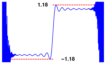
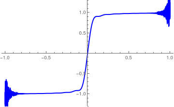
The graph clearly indicates on an existence of the Gibbs phenomenon at the origin. To investigate its presence, we increase the number of terms in the partial sum (5.8). Upon plotting with N = 22 terms, we observe divergence of Legendre series (5.2) at end points x = ±1. In order to eliminate the Gibbs phenomenon, we use Cesàro regularization
Theorem 6:
If function f(t) ∈ 𝔏²([−1, 1]) is square integrable and for some fixed point x ∈ (−1, 1) the following condition holds:
\[
\int_{-1}^1 \left[ \frac{f(x) - f(t)}{x-t} \right]^2 {\text d}t < \infty .
\]
Then the Legendre series \eqref{Eqlegendre.4} converges at this point.
Indeed, since |x| < 1, It follows from the Stieltjes--Bernstein inequality that the sequence \( \displaystyle \quad \left\{ \hat{P}_n (x) \right\} \quad \) of orthonormal polynomials Legendre is bounded. Therefore, we can apply the general theorem regarding convergence of Fourier series with respect to orthonormal polynomials. We formulate it again:
Theorem: If segment [𝑎, b] is finite and an auxiliary function \( \displaystyle \quad \varphi_x (t) = \frac{f(x) - f(t)}{x-t} \quad \)
belongs to 𝔏²([𝑎, b]) for fixed x ∈ [𝑎, b], and the sequence of orthonormal polynomials {pₙ) is bounded at point x, then the Fourier series with respect to these orthonormal polynomials converges to f(x).
The condition of Theorem 6 is satisfies when function f(t) has a
derivative at this point or if there exists an neighborhood of point x at which function f(t) satisfies Lipschitz condition with constant α > ½.
The following definition is used to measure quantitatively the uniform continuity of functions.
A function f : X → Y admits ω as (local) modulus of continuity at the point x in X if
\[
\omega (f, \delta ) = \sup_{|x - y| \le \delta} \left\vert f(x) - f(y) \right\vert .
\]
Theorem 7:
If function f(x) is continuous on interval [−1, 1] and its modulus of continuity satisfies the Dini condition on whole interval [−1, 1], that is,
\[
\lim_{n\to\infty} \omega \left( \frac{1}{2} , f \right) \ln n = 0 ,
\]
then its Legendre series \eqref{Eqlegendre.4} converges to f(x) at every point from open interval (−1, 1); moreover, it converges uniformly on every closed subinterval of (−1, 1).
Since function f(x) is continuous, we can apply the Lebesgue inequality
\[
\left\vert f(x) - \sum_{k=0}^n a_k \hat{P}_k (x) \right\vert \leqslant \left[ 1 + L_n (x) \right] E_n (f) ,
\tag{T7.1}
\]
where
\[
L_n (x) = \int_{-1}^1 \left\vert \sum_{k=0}^n \hat{P}_k (t) \, \hat{P}_k (x) \right\vert {\text d}t .
\tag{T7.2}
\]
Let us estimate integral (T7.2). for fixed x. We brake interval [−1, 1] into five pieces
\[
\left[ -1, -1 + \frac{\varepsilon}{2} \right] , \quad \left[ -1 + \frac{\varepsilon}{2} , x - \frac{1}{n} \right] ,
\]
and
\[
\left[ x - \frac{1}{n} , x + \frac{1}{n} \right] , \quad \left[ x + \frac{1}{n} , 1 - \frac{\varepsilon}{2} \right] ,\quad \left[ 1 - \frac{\varepsilon}{2} , 1 \right] .
\]
For x ∈ [−1 + ε, 1 −ε], we will denote these intervals by Δk, where k = 1, 2, 3, 4, 5. Then applying the Christoffel–Darboux formula for integral over first interval, we get
\begin{align*}
A_1 (x) &= \int_{\Delta_1} \left\vert \sum_{k=0}^n \hat{P}_k (x)\, \hat{P}_k (t) \right\vert {\text d} t
\\
& \leqslant c_1 \int_{\Delta_1} \left\vert \frac{\hat{P}_{n+1} \, \hat{P}_n (t) - \hat{P}_n (x)\, \hat{P}_{n+1} (t)}{x- t} \right\vert {\text d} t
\\
& \leqslant c_1 \left\vert \hat{P}_{n+1} (x) \right\vert \int_{\Delta_1} \frac{\left\vert \hat{P}_n (t) \right\vert}{| x - t |} \, {\text d} t
\\
& \qquad + c_1 \left\vert \hat{P}_{n} (x) \right\vert \int_{\Delta_1} \frac{\left\vert \hat{P}_{n+1} (t) \right\vert}{| x - t |} \, {\text d} t .
\end{align*}
Application of Bunyakovsky inequality yields
\[
\int_{\Delta_1} \frac{\left\vert \hat{P}_n (t) \right\vert}{| x - t |} \, {\text d} t \leqslant \left[ \int_{\Delta_1} \frac{{\text d}t}{|x-t|^2} \right]^{1/2} \left[ \int_{\Delta_1} \left\vert \hat{P}_n (t) \right\vert^2 {\text d} t \right]^{1/2}
\]
If t ∈ Δ₁ = [−1, −1 + ε/2], then |x − t| ≥ ε/2. Hence,
\[
\int_{\Delta_1} \frac{{\text d}t}{|x-t|^2} \leqslant c_2 \int_{\varepsilon /2}^{\varepsilon} \frac{{\text d}\tau}{\tau^2} = \frac{c_2}{\varepsilon} .
\]
Therefore, the right-hand part of last inequality does not exceed c₃/√ε.
Similarly, we can estimate the second integral and obtain
\[
A_1 (x) \leqslant \frac{c_4}{\sqrt{\varepsilon}\left( 1- x^2 \right)^{1/4}} \leqslant \frac{c_5}{\varepsilon^{3/4}} ,
\]
where constant c₅ does not depend on both, ε and n. A similar estimation is valid for the fifth integral.
Next, we get an estimation for the integral over second interval:
\[
A_2 (x) \leqslant \frac{c_6}{\sqrt{\varepsilon}} \int_{\Delta_2} \frac{{\text d}t}{x-t} \leqslant \frac{c_7}{\sqrt{\varepsilon}} \int_{1/n}^1 \frac{{\text d}\tau}{\tau} = \frac{c_7}{\sqrt{\varepsilon}} \, \ln n .
\]
A similar estimation holds for the integral over Δ₄.
Finally, we estimate the integral over the third interval [x − 1/n, x + 1/n]. We have
\[
A_3 (x) = \int_{\Delta_3} \left\vert \sum_{k=0}^n \hat{P}_k (x)\, \hat{P}_k (t) \right\vert {\text d}t \leqslant \frac{c_8 \left( n+1 \right)}{\sqrt{\varepsilon}} \int_{\Delta_3} {\text d}t \leqslant \frac{c_9}{\sqrt{\varepsilon}} .
\]
Uniting all these estimates, we obtain
\[
L_n (x) = \int_{-1}^1 \left\vert \sum_{k=0}^n \hat{P}_k (x)\, \hat{P}_k (t) \right\vert {\text d}t \leqslant \frac{c_{10} \ln n}{\varepsilon^{3/4}} , \quad x \in [-1+\varepsilon , 1-\varepsilon ] .
\]
This gives
\[
\lim_{n\to\infty} E_n (f)\,\ln n = 0 .
\]
Corollary:
If function f(x) is continuously differentiable on the closed interval [−1, 1] (this condition is usually abbreviated as f∈ℭ¹[−1, 1]), then its Legendre series \eqref{Eqlegendre.4} converges uniformly on this segment.
Using Bunyakovsky inequality, we get
\begin{align*}
L_n^2 &\leqslant 2 \int_{-1}^1 \left\vert \sum_{k=0}^n \hat{P}_k (x)\,\hat{P}_k (t) \right\vert^2 {\text d}t
\\
&= \sum_{k=0}^n \left\vert \hat{P}_k (x) \right\vert^2 \leqslant \sum_{k=0}^n (2k+1) \leqslant c\,n^2 .
\end{align*}
On the other hand, Jackson's inequality tells us that
\[
\lim_{n\to\infty} n\,E_n (f) = 0 .
\]
Hence, the right-hand side of
\[
\left\vert f(x) - \sum_{k=0}^n a_k \hat{P}_k (x) \right\vert \leqslant \left[ 1 + L_n (x) \right] E_n (f)
\]
tends to zero.
As we see from Example 5, Fourier--Legendre series \eqref{Eqlegendre.4} exhibits the Gibbs phenomenon at the points of discontinuity. This phenomenon indicates that restoring a function from its Legendre series is an ill-posed problem. A convenient regularization is based on Cesàro summation:
The following theorem provides a simple sufficient condition for uniform convergence. There are known some less restrictive conditions that guarantee uniform convergence; however, we do not pursue this topic.
Theorem 8:
If function f satisfies the https://en.wikipedia.org/wiki/Lipschitz_continuity">Lipschitz condition of order α > ½ on closed interval [−1, 1] (this condition is usually abbreviated as f∈ℭ¹[−1, 1]), then the corresponding Legendre series \eqref{Eqlegendre.4} converges to f(x) on this interval. Moreover,
\[
\left\vert f(x) - \sum_{k=0}^n a_k \hat{P}_k (x) \right\vert \leqslant \frac{c(\alpha )}{n^{\alpha - 1/2}} , \qquad x \in [-1, 1] .
\]
Suppose that f is an odd function on interval [−1, 1]. Since Pₙ(x) is odd when n is odd and Pₙ(x) is even when n is even, then the Legendre coefficients of f with even indices are all zero (c2j = 0). The Legendre series of f contains only odd indexed polynomials. Similarly, if f is an even function, then its Legendre series contains only even indexed polynomials.
Example 6:
Using the generating function and substitution \( p = 2t/(1 + t^2 ) , \) we get
The nth coefficient is then given by coef[[n]]. We sample a few values:
coef[[21]]
Out[34]= 180557/524288
coef[[22]]
Out[35]= 0
All the even coefficients are zero.
Now we define the mth partial sum, and then a graph of the mth partial sum, along with the original function. Because the coefficient of \( P_{0} (x)=1 \) is zero, we may start the sum over n with the n = 1 term. The given signum function is shown in blue and the partial sums in red.
You can use the slider to move through the graphs, and also to display a movie of the graphs. When you do this, you will see the familiar Gibbs overshoot/undershoot at the discontinuity. It is also observed a struggle to converge at the endpoints.
Numerical experiments show that the Legendre series (6.3) exhibits the Gibbs phenomenon at the origin---the point of discontinuity. The series also diverges at endpoints x = ±1. To eliminate unwanted overshoots and undershoots at the origin, we consider Cesàro approximation
The value of a Legendre polynomial Pₙ(x)
at x = 0 is 0 if n
is odd, and a non-zero value if n
is even, specifically \( \displaystyle \quad P_{2k} (0) = (-1)^k \frac{(2k)!}{2^{2k} (k! )^2} \quad \left( \mbox{or} \quad P_{2k} (0) = (-1)^k \frac{(2k-1)!!}{(2k)!!} \right) , \quad \)
with common values being P₀(0) = 1, P₂(0) = −½, P₄(0) = ⅜.
Legendre polynomials are either even or odd functions, so they only have non-zero values at x = 0
for even n.
where Wₙ is a polynomial of degree n, and the path of integration does not cross the cut of logarithm function. Mathematica has a dedicated command for this function: LegendreQ[n, x].
Example 13:
A German mathematician by the name of Eduard Heine (1821–1881) discovered in 1851 (Theorie der Anziehung eines Ellipsoids, (E. Heine, pp. 70-82), Journal für die reine und angewandte Mathematik, 42 (1851), 70--82) the Legendre expansion of 1/(z − u):
\[
\frac{1}{z-u} = \sum_{r\ge 0} a_r P_r (u) ,
\]
where coefficients are given by
\[
a_r = \frac{2r +1}{2} \int_{-1}^1 \frac{P_r (u)}{z-u}\,{\text d}u = \left( 2r + 1 \right) Q_r (z) .
\]
This suggests the formula
\[
\frac{1}{z-u} = \sum_{k\ge 0} \left( 2k+1 \right) Q_k (z)\,P_k (u)
\tag{22.1}
\]
The following proof of formula (22.1) is due to Christoffel (Über die Gaußische Quadratur und eine Verallgemeinerung derselben, (E.B. Christoffel, pp. 61-82), Journal für die reine und angewandte Mathematik, 55 (1858), 61--82).
When k ≥ 1, it follows from the recurrence relations
\begin{align*}
\left( 2k + 1 \right) z\, Q_k (z) &= \left( k+1 \right) Q_{k+1} (z) + k\, Q_{k-1} (z) ,
\\
\left( 2k + 1 \right) u\, P_k (u) &= \left( k+1 \right) P_{k+1} (u) + k\, P_{k-1} (u) ,
\end{align*}
that
\begin{align*}
& \left( 2k + 1 \right) \left( z-u \right) Q+k (z)\, P_k (u)
\\
& \qquad = \left( k+1 \right) \left\{ Q_{k+1} (z)\,P_k (u) - Q_k (z)\,P_{k+1} (u) \right\}
\\
& \qquad \quad -k \left\{ Q_k (z)\,P_{k-1} (u) - Q_{k-1} (z) P_k (u) \right\} .
\end{align*}
The corresponding formula when k = 0 is
\[
\left( z-u \right) Q_0 (z)\, P_0 (u) = \left\{ Q_1 (z)\, P_0 (u) - Q_0 (z)\, P_1 (u) \right\} + 1 .
\]
From these two formulas, we have by addition
\begin{align*}
&\sum_{k=0}^n \left( 2k + 1 \right) Q_k (z)\, P_k (u)
\\
& \qquad = \frac{1}{z-u} + \frac{n+1}{z-u} \left\{ Q_{n+1} (z)\, P_n (u) - Q_n (z)\, P_{n+1} (u) \right\} .
\end{align*}
To prove Heine's formula, we have therefore to show that
\[
\left( n+1 \right) \left\{ Q_{n+1} (z)\, P_n (u) - Q_n (z)\, P_{n+1} (u) \right\}
\]
tends to zero as n tends to infinity.
Now, if z = cosh(α + ⅉβ) where α > 0, ⅉ² = −1, and if ϕ is real, we get
\begin{align*}
&\left\vert z + \left( z^2 -1 \right)^{1/2} \cosh\phi \right\vert = \left\vert \cosh (\alpha + {\bf j}\beta ) + \sinh (\alpha + {\bf j}\beta )\,\cosh\phi \right\vert
\\
& \qquad = \left\{ \frac{1}{2} \left( \cosh 2\alpha + \cosh 2\beta \right) + \sinh 2\alpha \,\cosh\phi + \right.
\\
& \qquad \quad \left. + \frac{1}{2} \left( \cosh 2\alpha - \cosh 2 \beta \cosh^2 \phi \right)
\right\}^{1/2}
\\
& \qquad \ge \left\{ \cosh 2\alpha + \sinh 2\alpha\,\cosh\phi \right\} \ge e^{\alpha} .
\end{align*}
From Heine's integral
\[
Q_n (z) = \int_0^{\infty} \left[ z + \left( z^2 -1 \right)^{1/2} \cosh \phi \right]^{-n-1} {\text d}\phi ,
\]
it follows
\begin{align*}
\left\vert Q_n (z) \right\vert &= \left\vert \int_0^{\infty} \left[ z + \left( z^2 -1 \right)^{1/2} \cosh \phi \right]^{-n-1} {\text d}\phi \right\vert
\\
& \leqslant \int_0^{\infty} \left[ \cosh 2\alpha + \sinh 2\alpha\,\cosh\phi \right]^{-(n+1)/2} {\text d}\phi
\\
& \leqslant e^{-(n-1)\alpha} \int_0^{\infty} \left[ \cosh 2\alpha + \sinh 2\alpha \,\cosh\phi \right]^{-1} {\text d}\phi
\\
& \leqslant e^{-(n-1)\alpha} Q_0 (\cosh 2\alpha ) .
\end{align*}
Similarly, if u = cosh(γ + jδ), where γ > 0, and if θ is real, we have
\begin{align*}
&\quad \left\vert u + \left( u^2 -1 \right)^{1/2} \cos\theta \right\vert
\\
&= \left\vert \cosh (\gamma + {\bf j}\delta ) + \sinh (\gamma + {\bf j}\delta )\,\cos\theta \right\vert
\\
&= \left[ \frac{1}{2} \left( \cosh 2\gamma + \cos 2\delta \right) + \sinh 2\gamma \,\cos\theta + \frac{1}{2} \left( \cosh 2\gamma - \cos 2\delta \right) \cos^2 \theta \right]^{1/2}
\\
& \leqslant \left[ \cosh 2\gamma + \sinh 2\gamma \right]^{1/2} = e^{\gamma} ,
\end{align*}
and so, by Laplace's first integral
\[
P_n (z) = \frac{1}{\pi} \int_0^{\pi} \left[ z + \left( z^2 -1 \right)^{1/2} \cos\phi \right]^n {\text d}\phi ,
\]
we have
\[
\left\vert P_n (u) \right\vert = \frac{1}{\pi} \left\vert \int_0^{\pi} \left[ z + \left( z^2 -1 \right)^{1/2} \cos\phi \right]^n {\text d}\phi \right\vert \leqslant e^{n\gamma} .
\]
Now suppose that α is fixed and that ϵ is an arbitrary positive number less than α. Then when 0 ≤ γ ≤ &alpha − ϵ, we find that
\begin{align*}
&\left( n+1 \right) \left\vert Q_{n+1} (z)\, P_n (u) - Q_n (z)\, P_{n+1} (u) \right\vert
\\
& \leqslant \left( n+1 \right) \left[ e^{-n\alpha} Q_0 (\cosh 2\alpha ) \, e^{n\gamma} + e^{-(n-1) \alpha} Q_0 (\cosh 2\alpha )\, e^{(n+1)\gamma} \right]
\\
&= \left( n+1 \right) Q_0 (\cosh 2\alpha )\, e^{n\left( \gamma - \alpha \right)} \left[ 1 + e^{2\alpha} \right]
\\
& < \left( n+1 \right) Q_0 (\cosh 2\alpha )\,e^{-n\epsilon} \left[ 1 + e^{2\alpha} \right] .
\end{align*}
This last expression does not depend on β, γ, or δ, and tends to zero as n tends to infinity. It follows that the series
\[
\sum_{n\ge 0} \left( 2n+1 \right) Q_n (z)\, P_n (u)
\]
converges uniformly with respect to β, γ, and δ, and has sum 1/(z − u).
The simplest way of stating this result is to use geometrical language. If we keep α fixed and vary β, the point z = cosh(α + jβ) traces out an ellipse with foci at the points of affix ±1 and major axis of length 2 cosh2α. The condition 0 ≤ γ ≤ α − ϵ means that u = cosh(γ + ⅉδ) lies within or on the smaller confocal ellipse of major axis 2 cosh(α − ϵ). This result can be reformulated as follows:
The series
\[
\sum_{n\ge 0} \left( 2n + 1 \right) Q_n (z)\, P_n (u)
\]
converges uniformly with respect to z and u when z lies on a fixed ellipse C with foci at the points of affix ±1 and u lies in any closed domain definitely within C. The sum of the series is 1/(z − u).
■
End of Example 13
Theorem 22 (Neumann):
If f(z) is an analytic function regular within and on an ellipse C with foci at the points of affix ±1, it can be expanded as a series of Legendre polynomials
\[
f(x) = \sum_{n\ge 0} c_n P_n (z)
\]
that converges uniformly when z lies within or on a smaller ellipse C₁, confocal with C.
For if u is any point within or on C₁, we have
\begin{align*}
f(u) &= \frac{1}{2\pi{\bf j}} \oint_C f(z)\,\frac{{\text d}z}{z-u}
\\
&= \frac{1}{2\pi{\bf j}} \oint_C f(z)\,\sum_{n\ge 0} \left( 2n+1 \right) Q_n (z)\,P_n (u)\,{\text d}z
\\
&= \frac{1}{2\pi{\bf j}}\, \sum_{n\ge 0} \oint_C f(z)\,\left( 2n+1 \right) Q_n (z)\,P_n (u)\,{\text d}z ,
\end{align*}
the inversion of the order of integration being valid since the infinite series under the sign of integration is uniformly convergent with respect to z and u when z lies on C. Then it follows that f(u) can be expressed as a uniformly convergent series
\[
f(u) = \sum_{n\ge 0} c_n P_n (u) ,
\]
where
\[
c_n = \frac{2n+1}{2\pi{\bf j}} \oint_C f(z)\,Q_n (z)\,{\text d} z.
\]
This completes the proof of Karl Neumann's expansion theorem.
then eigenfunction expansion \eqref{Eqlegendre.11} converges uniformly.
Suppose that f(z) is an analytic function regular in an annulus bounded externally by an ellipse C₂ with foci at the points of affix ±1, and internally by a smaller confocal ellipse C₁. Show that f(z) can be expanded as a series of the form
\[
f(z) = \sum_{n\ge 0} a_n P_n (z) + \sum_{n\ge 0} b_n Q_n (z) ,
\]
where
\begin{align*}
a_n &= \frac{2n+1}{2\i{\bf j}} \oint_{C_2} f(z)\,Q_n (z)\,{\text d} z ,
\\
b_n &= \frac{2n+1}{2\i{\bf j}} \oint_{C_1} f(z)\,P_n (z)\,{\text d} z .
\end{align*}
Abramowitz, M. & Stegun, I. A., Handbook of Mathematical Functions: with Formulas, Graphs, and Mathematical Tables, (Dover Books on Mathematics), 1965.
Askey, R., Orthogonal Polynomials and Special Functions, AMS, Contemporary Mathematics,
Volume: 471; 2008.
Bera, R.K. and Ghodadra, B.L.,
Convergence Rate of Fourier–Legendre Series of Functions of Generalized Bounded Variation,
Mathematical Notes, 116 (2024), 168–181.
Bera, R.K. and Ghodadra, B.L.,
Rate of convergence Rate of Fourier–Legendre Series of Functions of class (nα)BVp[−1, 1],
Acta et Commentationes Universitatis Tartuensis de mathematica, Volume 28, Number 2, 2024; Available online at https://ojs.utlib.ee/index.php/ACUTM
Bojanić, R. and Vuilleumier, M.,
On the Rate of Convergence of Fourier–Legendre Series of Functions of Bounded Variation,
Journal of Approximation Theory, 31 (1981), 67–79.
Courant, R. and Hilbert, D., Methods of Mathematical Physics, Vol. I, Wiley-VCH, 1989.
Christoffel, E. B. (1858), "Über die Gaußische Quadratur und eine Verallgemeinerung derselben.", Journal für die Reine und Angewandte Mathematik (in German), 55: 61–82, doi:10.1515/crll.1858.55.61
Gasper — Positive Kernels and Orthogonal Polynomials,
Goginava, U.,
Classes of Functions of Bounded Generalized Variation,
arXiv:1210.2511
Hobson, E.W., The Theory of Spherical and Ellipsoidal Harmonics, Cambridge University Press, 2012.
Muckenhoupt, B. Mean convergence of orthogonal series. Transactions of the American Mathematical Society, 147 (1970), 419-431.
DOI: https://doi.org/10.1090/S0002-9947-1970-99933-9
Stein, E.M. and Weiss, G., Introduction to Fourier Analysis on Euclidean Spaces, Princeton University Press, 1971.
Szegő, G., Orthogonal Polynomials, American Mathematical Society, 1939.
Return to Mathematica page
Return to the main page (APMA0340)
Return to the Part 1 Matrix Algebra
Return to the Part 2 Linear Systems of Ordinary Differential Equations
Return to the Part 3 Non-linear Systems of Ordinary Differential Equations
Return to the Part 4 Numerical Methods
Return to the Part 5 Fourier Series
Return to the Part 6 Partial Differential Equations
Return to the Part 7 Special Functions


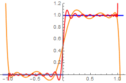
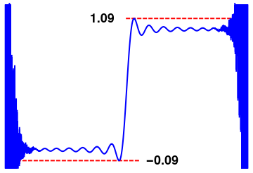
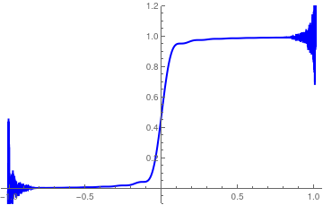


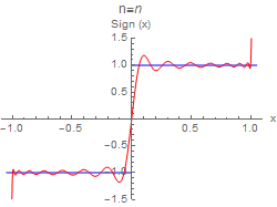 DynamicModule[{mangraph, i}, Do[mangraph[i] = legraph[i], {i, 1, 55, 2}]; Manipulate[mangraph[i], {i, 1, 51, 2}]]You can use the slider to move through the graphs, and also to display a movie of the graphs. When you do this, you will see the familiar Gibbs overshoot/undershoot at the discontinuity. It is also observed a struggle to converge at the endpoints.Module[{a}, coef = {}; Do[coef = Append[coef, (LegendreP[x - 1, 0] - LegendreP[x + 1, 0])], {x, 1, 100}]] legsum[m_, x_] := Module[{a}, -Sum[N[coef[[a]]]*LegendreP[a, x], {a, 1, m}]] leg[x_] = Piecewise[{{1, -1 <= x < 0}, {-1, 0 < x <= 1}}]; legraph[m_] := Plot[{leg[x], legsum[m, x]}, {x, -1, 1}, PlotRange -> {-1.5, 1.5}, PlotStyle -> {{RGBColor[0, 0, 1], Thickness[0.005]}, {RGBColor[1, 0, 0], Thickness[0.005]}}] legraph[10] legraph[100]