This section is devoted to expansions of real-valued functions into series over
Laguerre polynomials
\[
f(x) = \sum_{k\ge 0} f_k L_k (x) , \qquad f_k = \int_0^{\infty} L_k (x) \,e^{-x} f(x) \, {\text d} x ,
\tag{7}
\]
and Sonin polynomials
\[
f(x) = \sum_{k\ge 0} f_k^{(\alpha )} L_k^{(\alpha )} (x) , \qquad f_k^{(\alpha )} = \frac{k!}{\Gamma (k + \alpha + 1)}\int_0^{\infty} L_k^{(\alpha )} (x) \,e^{-x} x^{\alpha} f(x) \, {\text d} x , \qquad k = 0,1,2,\ldots .
\tag{8}
\]
It is known that these series converge in 𝔏² sense for functions
f ∈ 𝔏²(ℝ
+ ,
x α e −x ).
We do not discuss a delicate topic of pointwise and uniform convergence of these series. Instead, we present some examples of these series for demonstration.
Laguerre's polynomials ,
\begin{equation} \label{EqLaguerre.1}
L_n (x) = \sum_{k=0}^n (-1)^k \binom{n}{k} \frac{x^k}{k!} , \qquad n=0,1,2,\ldots ,
\end{equation}
are eigenfunctions of the singular Sturm--Liouville problem on the half-line (0, ∞):
\[
x\,y'' + \left( 1 -x \right) y' + \lambda\,y = 0, \qquad \lambda = n.
\]
Here
\( \displaystyle \binom{n}{k} = \frac{n^{\underline{k}}}{k!} = \frac{n \left( n-1 \right) \left( n-2 \right) \cdots \left( n-k+1 \right)}{1\cdot 2 \cdot 3 \cdots k} \) is the
binomial coefficient .
The polynomials \eqref{EqLaguerre.1} were invented by the Russian mathematician
Pafnuty Chebyshev (1821--1894) in 1859.
Therefore, these polynomials were known in nineteen century as Chebyshev--Laguerre polynomials.
The Laguerre equation has one regular singular point at the origin and irregular singular point at infinity. So the
Laguerre polynomial is a bounded at the origin solution to the Chebyshev--Laguerre equation
\begin{equation} \label{EqLaguerre.2}
x\,y'' + \left( 1-x \right) y' +n\,y =0, \qquad\mbox{or in self-adjoint form} \qquad \frac{{\text d}}{{\text d} x} \left( x\,e^{-x} \,y' \right) + n\,e^{-x}\,y =0 , \qquad x\in (0,\infty ).
\end{equation}
In 1880, the Russian mathematician
Nikolay Yakovlevich Sonin (1849--1915) introduced a generalization of the Laguerre equation:
\begin{equation} \label{EqLaguerre.3}
x\,y'' + \left( 1-x + \alpha \right) y' +n\,y =0, \qquad\mbox{or in self-adjoint form} \qquad \frac{{\text d}}{{\text d} x} \left( x^{1 + \alpha} e^{-x} \,y' \right) + n\, x^{\alpha} e^{-x}\,y =0 , \qquad x\in (0,\infty ),
\end{equation}
where α > −1 is a real parameter.
It has a polynomial solution
\begin{equation} \label{EqLaguerre.4}
L_n^{(\alpha )} (x) = \sum_{k=0}^n \frac{\Gamma (n+ \alpha + 1)}{\Gamma (k + \alpha + 1)} \cdot \frac{(-x)^k}{k! \left( n-k \right) !} = \frac{1}{n!} \sum_{k=0}^n \frac{\Gamma (n+ \alpha + 1)}{\Gamma (k + \alpha + 1)} \binom{n}{k} (-x)^k ,
\end{equation}
known as the
Sonin polynomial of degree
n . This function, also denoted as
L n (α,
x ), is usually referred to as the
generalized or
associated Laguerre polynomial .
A definition of orthogonality requires a special bilinear form, called an
inner product , denoted with angle brackets such as in ⟨ 𝑎,
b ⟩. A vector space of functions equipped with an inner product is called a
Hilbert space subject that it is
complete . An importatnt example of Hilbert space presents the space of square Lebesque integrabler real- or complex-valued functions on some interval, denoted by 𝔏². Then the inner product (with weight ρ ≥ 0)
\[
\left\langle f(x), g(x) \right\rangle = \int_a^b \overline{f(x)}\,g(x)\,\rho(x)\,{\text d}x ,
\]
generats a
norm \( \| f \| = \left\langle f(x), f(x) \right\rangle^{1/2} . \) Here
\( \overline{f(x)} \) denotes the complex conjugate of
f (
x ). In particular, we are intereted in a semi-infinite interval (when 𝑎 = 0 and
b = +∞) and an inner product involving a weight function ρ(
x ≥ 0:
\[
\left\langle f(x), g(x) \right\rangle = \int_0^{\infty} \overline{f(x)}\,g(x)\,x^{\alpha} e^{-x} {\text d}x \qquad \Longrightarrow \qquad \| f \|^2 = \left\langle f(x), f(x) \right\rangle ,
\]
where α > −1. The corresponded complete space is denoted as
𝔏²(ℝ
+ ;
x α e −x ). A Hilbert space is always
complete meaning that every
Cauchy sequence converges.
The Sonin polynomials or associated Laguerre polynomials are orthogonal over [0, ∞) with respect to the weighting function
\( \rho (x) = x^{\alpha} e^{-x} : \)
\begin{equation} \label{EqLaguerre.5}
\left\langle L_n^{(\alpha )} (x) , L_m^{(\alpha )} (x) \right\rangle = \int_0^{\infty} x^{\alpha} e^{-x} L_n^{(\alpha )} (x) \, L_m^{(\alpha )} (x) \,{\text d}x = \frac{\Gamma (n+\alpha + 1)}{n!}\, \delta_{n,m} ,
\end{equation}
where
\( \Gamma (\nu ) = \int_0^{\infty} t^{\nu -1} e^{-t} {\text d}t \) is the
gamma function of
Euler and
\[
\delta_{n,m} = \begin{cases}
0, & \ \mbox{when} \quad n \ne m , \\
1, & \ \mbox{for} \quad n = m,
\end{cases}
\]
is the
Kronecker delta symbol. In particular,
\begin{equation} \label{EqLaguerre.6}
\left\langle L_n (x) , L_m (x) \right\rangle = \int_0^{\infty} e^{-x} L_n (x) \, L_m (x) \,{\text d}x = \delta_{n,m} .
\end{equation}
Note that Hilbert spaces 𝔏²(ℝ
+ ;
x α e −x ) or 𝔏²(ℝ
+ ;
e −x ) contain unbounded (not integrable) functions on semi-infinite line ℝ
+ = [0, ∞), including polynomials.
Arbitrary function
f ∈ 𝔏²((0,∞);
e −x ), for which the integral
\[
\| f \|^2 = \int_0^{\infty} e^{-x} |f(x)|^2 {\text d} x < \infty
\]
is finite, can be expanded into Fourier--Laguerre series:
\begin{equation} \label{EqLaguerre.7}
f(x) = \sum_{i\ge 0} f_i L_i (x) , \qquad f_i = \int_0^{\infty} L_i (x) \,e^{-x} f(x) \, {\text d} x ,
\end{equation}
which converges in 𝔏
p (ℝ
+ ,
e −x ) for
\( p \in \left( \frac{4}{3} , 4 \right) . \)
Such expansion is based on the orthogonal property of Laguerre polynomials, Eq.\eqref{EqLaguerre.6}.
More generally, introducing the inner product and norm in 𝔏²((0,∞, x α e −x )
\[
\left\langle f(x), g(x) \right\rangle = \int_0^{\infty} x^{\alpha} e^{-x} f(x)\, g(x)\,{\text d} x \qquad \Longrightarrow \qquad \| f \|^2 = \int_0^{\infty} x^{\alpha} e^{-x} f^2(x)\,{\text d} x ,
\]
we expand a real-valued function
f (
x )∈𝔏²(ℝ
+ ,
x α e −x ) into
Sonin series
\begin{equation} \label{EqLaguerre.8}
f(x) = \sum_{k\ge 0} f_k^{(\alpha )} L_k^{(\alpha )} (x) , \qquad f_k^{(\alpha )} = \frac{k!}{\Gamma (k + \alpha + 1)}\int_0^{\infty} L_k^{(\alpha )} (x) \,e^{-x} x^{\alpha} f(x) \, {\text d} x , \qquad k = 0,1,2,\ldots .
\end{equation}
Theorem (
Parseval ):
Let
f : [0, ∞) → ℝ (or ℂ) belongs to the
Hilbert space 𝔏²(ℝ
+ ,
x α e −x ). Then
Parseval's identity holds
\[
\int_0^{\infty} \left\vert f(x) \right\vert^2 x^{\alpha} e^{-x} {\text d}x = \sum_{n\ge 0} \left( f_k^{(\alpha )} \right)^2 \frac{\Gamma (n+\alpha +1)}{n!} = \sum_{n\ge 0} \frac{n!}{\Gamma (n+\alpha +1)} \,\left\langle f(x), L_n^{(\alpha )} (x) \right\rangle^2 .
\]
If function
f ∈𝔏²((0,∞);
x α e −x ) is sufficiently smooth, then coefficients in Eq.\eqref{EqLaguerre.8} can be expressed as
\begin{equation} \label{EqLaguerre.9}
f_n = \frac{1}{\| L_n (\alpha ,x \|^2}\,\langle f, L_n^{(\alpha )} \rangle = \frac{n!}{\Gamma (n + \alpha + 1)}\,\int_0^{\infty} f(x) \, L_n^{(\alpha )} (x)\, x^{\alpha} e^{-x} {\text d} x = \frac{1}{\| L_n (\alpha ,x \|^2} \cdot \frac{(-1)^n}{n!}\,\int_0^{\infty} f^{(n)} (x) \, x^{n+\alpha} e^{-x} {\text d} x .
\end{equation}
When f (x ) is a polynomial of degree k < n , then
\[
\left\langle f(x), L_n^{(\alpha )} (x) \right\rangle = \int_0^{\infty} f(x) \, L_n^{(\alpha )} (x)\, x^{\alpha} e^{-x} {\text d} x = 0.
\]
The first example follows from the generating function:
\[
x^{-\alpha} e^x \Gamma (\alpha , x) = \sum_{n\ge 0} \frac{L_n^{(\alpha )} (x)}{n+1} ,
\]
where
\[
\Gamma (\nu , A) = \int_A^{\infty} t^{\nu -1} e^{-t} {\text d} t
\]
is
incomplete gamma function . This formula can be used for numerical evaluation of the
incomplete gamma function as well as the complete gamma function.
Example 1: Gamma function is expanded into Laguerre series
Example 1: Exponential integral :
\[
\Gamma (0 , x) = \int_x^{\infty} t^{-1} e^{-t} {\text d}t = -\mbox{Ei}(-x) = e^{-x} \sum_{n\ge 0} \frac{L_n (x)}{n+1} .
\]
Of course,
Mathematica has a dedicated command,
ExpIntegralEi , but we apply the Laguerre series for its approximation. So we build partial sums:
We plot the exponential integral (in blue) and its Laguerre approximations with 10 and 20 terms:
S10[x_] = Exp[-x]*Sum[LaguerreL[n, x]/(n + 1), {n, 0, 10}];
Laguerre approximations with 10 and 20 terms.
Mathematica code.
We also check the accuracy by evaluating approximate values at
x = 5.0:
S10[5.0]
0.0031435
S20[5.0]
0.00191203
-ExpIntegralEi[-5.0]
0.0011483
NIntegrate[Exp[-x]/x, {x, 5.0, Infinity}]
0.0011483
So 20-term Laguerre approximation gives 3 correct decimal places.
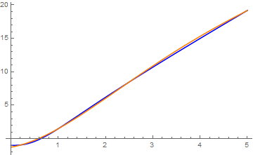
We expand the incomplete gamma function into Laguerre series:
\[
\Gamma (\alpha , x) = \int_{x}^{\infty} t^{\alpha -1} e^{-t} {\text d} t = x^{\alpha} e^{-x} \sum_{n\ge 0} \frac{L_n^{(\alpha )} (x)}{n+1}
\]
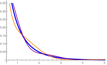
We take α = 3/2, and use the Sonin expansion:
\[
\Gamma \left(\frac{3}{2} , x\right) = \int_{x}^{\infty} t^{1/2} e^{-t} {\text d} t = x^{3/2} e^{-x} \sum_{n\ge 0} \frac{L_n^{(3/2 )} (x)}{n+1} .
\]
We plot the incomplete gamma function (in blue) and its Sonin approximation (in orange) with 50 terms along with the corresponding Cesàro regularization (in purple):
\[
C50(x) = x^{3/2} e^{-x} \sum_{n= 0}^{50} \frac{L_n^{(3/2 )} (x)}{n+1} \left( 1 - \frac{n}{51} \right) .
\]
S50[x_] =
x^(3/2)*Exp[-x]*Sum[LaguerreL[n, 3/2, x]/(n + 1), {n, 0, 50}];
Sonin and corresponding Cesàro approximations with 50 terms.
Mathematica code.
We also check the accuracy by evaluating approximate values at
x = 5.0:
S50[5.0]
-0.0121446
C50[5.0]
0.0187587
Gamma[3/2, 5.0, Infinity]
0.0164538
NIntegrate[t^(1/2)*Exp[-t], {t, 5.0, Infinity}]
0.0164538
So we see that 50-term Sonin approximation has a poor accuracy. However, its Cesàro regularization gives much better approximation.
■
Example 2: Exponential functions are expended into Laguerre series
Example 2: \( w = a/(a+1) , \) we find
\[
e^{-ax} = \frac{1}{(1+a)^{1 + \alpha}} \,\sum_{k\ge 0} \left( \frac{a}{1+a} \right)^k L_k^{(\alpha )} (x) \qquad \Re\alpha > ½.
\]
In particular,
\[
e^{-x} = \sum_{k\ge 0} \frac{1}{2^{k + \alpha + 1}} \, L_k^{(\alpha )} (x) , \qquad 0 < x < \infty .
\]
Multiplying the former series by
\( (a+1)^{\alpha -1} \) and integrate, we get
\[
x^{-\alpha} e^x \Gamma (\alpha , x) = \sum_{n\ge 0} \frac{1}{n+1} \, L_n^{(\alpha )} (x) , \qquad \alpha > -1,
\]
where
\( \displaystyle
\Gamma (\nu , A) = \int_A^{\infty} t^{\nu -1} e^{-t} {\text d} t
\)
is the
incomplete gamma function .
With exponential function, we verify Parseval's identiy:
\[
\int_0^{\infty} \left( e^{-x} \right)^2 e^{-x} {\text d} x = \int_0^{\infty} e^{-3x} {\text d} x = \frac{1}{3} = \sum_{k\ge 0} \left( \frac{1}{2^{k + 1}} \right)^2 .
\]
Integrate[Exp[-3*x], {x, 0, Infinity}]
1/3
Sum[1/4^(k + 1), {k, 0, Infinity}]
1/3
We also have expansion for the natural logarithm function:
\[
\ln x = \frac{\Gamma' (\alpha +1)}{\Gamma (\alpha +1)} - \Gamma (\alpha +1) \sum_{n\ge 1} \frac{(n-1)!}{\Gamma (\alpha +n +1)}\, L_n^{(\alpha )} (x) .
\]
Here the logarithmic derivative of the gamma function
\[
\psi (x) = \frac{\text d}{{\text d}x}\,\ln\Gamma (x) = \frac{\Gamma' (x)}{\Gamma (x)}
\]
is called the
digamma function .
Mathematica has a dedicated command:
PolyGamma[x]. For α = 0, we get the Laguerre series
\[
\ln x = \psi (1) - \sum_{n\ge 1} \frac{1}{n}\, L_n (x) .
\]
We plot two Laguerre approximations with 10 and 50 terms.
ln[n_] = PolyGamma[1] - Sum[(1/k)*LaguerreL[k, x], {k, 1, n}];
Laguerre approximations of the logarithm function with 10 and 50 terms.
Mathematica code.
We verify Parseval's identity for logarithmic function expansion:
\[
\int_0^{\infty} \left( \ln x \right)^2 e^{-x} {\text d}x = \left( \psi (1) \right)^2 + \sum_{n\ge 1} \frac{1}{n^2} .
\]
Mathematica confirms
NIntegrate[(Log[x])^2 *Exp[-x], {x, 0, Infinity}]
1.97811
N[PolyGamma[1]^2 + Sum[1/n^2, {n, 1, Infinity}]]
1.97811
Now we check Parseval's identity for Sonin expansion:
\[
\| \ln x \|^2 = \int_0^{\infty} \left( \ln x \right)^2 x^{\alpha} e^{-x} {\text d}x = \left( \Gamma (\alpha +1)\,\psi (\alpha +1) \right)^2 + \Gamma (\alpha +1)^2 \sum_{n\ge 1} \frac{(n-1)!}{\Gamma (n+\alpha +1)\,n} \approx 0.829627 .
\]
Upon taking α = ½, we use
Mathematica
NIntegrate[(Log[x])^2 *Exp[-x]*Sqrt[x], {x, 0, Infinity}]
0.829627
N[(Gamma[3/2]*PolyGamma[3/2])^2 + (Gamma[3/2])^2 *
Sum[Factorial[n - 1]/Gamma[3/2 + n]/n, {n, 1, Infinity}]]
0.829493
■
Example 3: Cubic function
Example 3: \( f(x) = 4\,x^3 -1 . \) This function has a finite square norm with weight \( e^{-x} : \)
\[
\| 4\,x^3 -1 \|_2^2 = \int_0^{\infty} \left( 4\,x^3 -1 \right)^2 \, e^{-x} \, {\text d} x = 11473.
\]
Therefore, this function can be expanded into convergent Laguerre series (which is actually a finite sum):
\[
4\,x^3 -1 = \sum_{k\ge 0} c_k L_k (x) ,
\]
where
\[
c_0 = \int_0^{\infty} \left( 4\,x^3 -1 \right) \,e^{-x} \, {\text d} x = 23 , \quad c_1 = -72, \quad c_2 =72, \quad c_3 = -24 .
\]
All other coefficients are zeroes, and we get the identity:
\[
4\,x^3 -1 = 23\,L_0 (x) -72\,L_1 (x) + 72\,L_2 (x) -24\,L_3 (x) ,
\]
■
Example 4: Arbitrary power function
Example 4: \( f(x) = x^p , \) where parameter p satisfies the condition:
\[
\begin{split}
p & > - \frac{1}{2} \left( \alpha + \frac{3}{2} \right) \quad \mbox{if} \quad \alpha > 0, \\
p & > - \left( \frac{\alpha}{2} + \frac{1}{4} \right) \quad \mbox{if} \quad -1 < \alpha \le 0. \end{split}
\]
To answer this question, we need to find coefficients c k in the Laguerre expansion:
\[
c_k = \int_0^{\infty} x^p e^{-x} L_k (x)\,{\text d} x = \frac{1}{k!} \, \int_0^{\infty} x^p \,\frac{{\text d}^k}{{\text d} x^k} \left( x^k e^{-x} \right) , \quad k=0,1,2,\ldots .
\]
Starting with
k = 0 , we have
\[
c_0 = \int_0^{\infty} x^p e^{-x} \,{\text d} x = \Gamma (p+1) ,
\]
where Γ(ν) is the
gamma function of
Euler . For
k > 0 , we integrate by parts in the integral
\begin{align*}
c_k &= \frac{1}{k!} \, \int_0^{\infty} x^p \,\frac{{\text d}^k}{{\text d} x^k} \left( x^k e^{-x} \right) \,{\text d} x = \left. \frac{1}{k!} \, x^p \,\frac{{\text d}^{k-1}}{{\text d} x^{k-1}} \left( x^k e^{-x} \right) \right\vert_{x=0}^{\infty} - \frac{p}{k!} \, \int_0^{\infty} x^{p-1} \,\frac{{\text d}^{k-1}}{{\text d} x^{k-1}} \left( x^k e^{-x} \right) \,{\text d} x
\\
&= -\left. \frac{p}{k!} \, x^{p-1} \,\frac{{\text d}^{k-2}}{{\text d} x^{k-2}} \left( x^k e^{-x} \right) \right\vert_{x=0}^{\infty} + \frac{p(p-1)}{k!} \, \int_0^{\infty} x^{p-2} \,\frac{{\text d}^{k-2}}{{\text d} x^{k-2}} \left( x^k e^{-x} \right) \,{\text d} x
\\
&= (-1)^k \,\frac{1}{k!} \, p^{\underline{k}} \, \Gamma (p+1) = \Gamma (p+1) (-1)^k \binom{p}{k} ,
\end{align*}
where
\( p^{\underline{k}} = p(p-1) \cdots (p-k+1) \) is
k th
falling factorial . Hence, the Fourier-Laguerre series expansion of the power function is given by
\[
x^p = \Gamma (p+1) + \Gamma (p+1) \,\sum_{k\ge 1} \frac{(-1)^k}{k!} \, p^{\underline{k}} \, L_k (x) = \Gamma (p+1) + \Gamma (p+1) \,\sum_{k\ge 1} (-1)^k \binom{p}{k} L_k (x) .
\]
We check some first coefficients with
Mathematica :
Assuming[p > 0,
Integrate[x^p*Exp[-x]*LaguerreL[1, x], {x, 0, Infinity}]]
Gamma[1 + p] - Gamma[2 + p]
Assuming[p > 0,
Integrate[x^p*Exp[-x]*LaguerreL[2, x], {x, 0, Infinity}]]
1/2 (-1 + p) p Gamma[1 + p]
Assuming[p > 0,
Integrate[x^p*Exp[-x]*LaguerreL[3, x], {x, 0, Infinity}]]
-(1/6) (-2 + p) (-1 + p) p Gamma[1 + p]
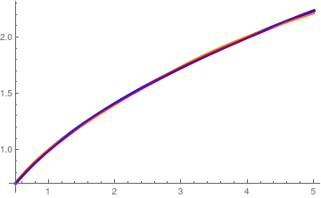
We plot two Laguerre approximations of the square root function with 10 and 50 terms for p = ½.
root[n_] =
Gamma[3/2] +
Gamma[3/2]*
Sum[((-1)^k *Binomial[1/2 , k]*LaguerreL[k, x], {k,
1, n}];
Laguerre approximations of the square root function with 10 and 50 terms.
Mathematica code.
We check Parseval's identity for the square root:
\[
\| \sqrt{x} \|^2 = \int_0^{\infty} x\,e^{-x} {\text d}x = 1 = \Gamma^2 (3/2) \left[ 1 + \sum_{k\ge 1} \binom{1/2}{k}^2 \right] .
\]
Integrate[x*Exp[-x], {x, 0, Infinity}]
1
N[Gamma[3/2]^2*(1 + Sum[Binomial[1/2, k]^2, {k, 1, Infinity}])]
1.
If p is a positive integer, the above series becomes a polynomial of degree p because falling factorial \( p^{\underline{k}} =0 \) for k > p . Also \( \Gamma (p+1) = p! \) for positive integer p .
In particular,
\[
x^n = n! \,\sum_{k=0}^n (-1)^k \binom{n+\alpha}{n-k} \, L_k^{(\alpha )} (x) .
\]
The binomial coefficients have the parametrization
\[
\binom{n+x}{n} = \sum_{k=0}^n \frac{\alpha^k}{k!} \, L_{n-k}^{(x+k )} (\alpha ) .
\]
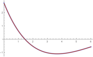
Example 5: Rational function
Example 5: \( \displaystyle f(x) = \frac{4\,x^3 -1}{x^2 +1} . \) This function has a finite square norm with weight \( e^{-x} : \)
\[
\left\| \frac{4\,x^3 -1}{x^2 +1} \right\|_2^2 = \int_0^{\infty} \left( \frac{4\,x^3 -1}{x^2 +1} \right)^2 \, e^{-x} \, {\text d} x \approx 21.3606.
\]
Therefore, this function can be expanded into convergent Laguerre series
\[
\frac{4\,x^3 -1}{x^2 +1} = \sum_{k\ge 0} c_k L_k (x) ,
\]
where
\begin{align*}
c_0 &= \int_0^{\infty} \left( \frac{4\,x^3 -1}{x^2 +1} \right) \, e^{-x} \, {\text d} x \approx 2.00504,
\\
c_1 &= \int_0^{\infty} \left( \frac{4\,x^3 -1}{x^2 +1} \right) \, e^{-x} \,L_1 (x) \, {\text d} x \approx -4.13738,
\\
c_2 &= \int_0^{\infty} \left( \frac{4\,x^3 -1}{x^2 +1} \right) \, e^{-x} \,L_2 (x) \, {\text d} x \approx 0.217678,
\\
c_3 &= \int_0^{\infty} \left( \frac{4\,x^3 -1}{x^2 +1} \right) \, e^{-x} \,L_3 (x) \, {\text d} x \approx 0.260623,
\end{align*}
and so on, getting
\( c_4 \approx 0.223731, \ c_5 \approx 0.17164. \) Now we build Laguerre approximation with six terms:
c3 = NIntegrate[
LaguerreL[3, x]*(4*x^3 - 1)*Exp[-x]/(x*x + 1), {x, 0, Infinity}]
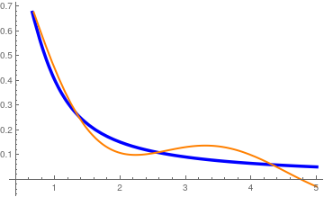
Example 5B: \( \displaystyle g(x) = \frac{x^2 +1}{4\,x^3 +1} \) that decays at infinity. First, we check whether the given function belongs to the Hilbert space
𝔏²(ℝ+ , e −x )
NIntegrate[(x^2 + 1)/(4*x^3 + 1)^2*Exp[-x], {x, 0, Infinity}]
0.424348
Then we calculate first few coefficients in Fourier--Laguerre series
c0 = NIntegrate[(x^2 + 1)/(4*x^3 + 1)*Exp[-x], {x, 0, Infinity}]
Then we build a 10-term approximation
rat[x_] = c0+N[Sum[c[[n]]*LaguerreL[n, x], {n, 1, 10}]];
We plot a Laguerre approximations of the rational function with 10 terms.
Plot[{(x^2 + 1)/(4*x^3 + 1), rat[x]}, {x, 0.4, 5},
PlotStyle -> {{Thickness[0.01], Blue}, {Thick, Orange}}]
Laguerre approximations of the rational function with 10 terms.
Mathematica code.
Finally, we check validity of Paeseval's identity:
\[
0.424348 = \| g(x) \|^2 = \int_0^{\infty} \left( \frac{x^2 +1}{4\,x^3 +1} \right)^2 e^{-x} {\text d}x = \sum_{n\ge 0} c_n^2 .
\]
N[Sum[c[[n]]^2, {n, 1, 10}]] + c0^2
0.485588
■
Example 6: Bessel function expansion
Example 6:
\[
F(x) = \left( xt \right)^{-\alpha /2} J_{\alpha} \left( 2 \sqrt{xt} \right) , \qquad a > 0, \quad \alpha > -1, \quad x > 0.
\]
Expanding this function into Sonin polynomials, we obtain
\[
\left( xt \right)^{-\alpha /2} J_{\alpha} \left( 2 \sqrt{xt} \right) = e^{-t} \sum_{n\ge 0} \frac{t^n}{\Gamma \left( \alpha + n +1 \right)}\,
L_n^{(\alpha )} (x) .
\]
So
\[
e^t \left( tx \right)^{-\alpha /2} J_{\alpha} \left( 2\sqrt{xt} \right) = \sum_{n\ge 0} \frac{L_n^{(\alpha )} (x)}{\Gamma (n+ \alpha + 1)} \, t^n .
\tag{6.1}
\]
In particular,
\[
\left( x \right)^{-\alpha /2} J_{\alpha} \left( 2\sqrt{x} \right) e = \sum_{n\ge 0} \frac{L_n^{(\alpha )} (x)}{\Gamma (n+ \alpha + 1)} .
\tag{6.2}
\]
For α = 0, we have
\[
J_{0} \left( 2\sqrt{x} \right) e = \sum_{n\ge 0} \frac{L_n (x)}{n!} .
\tag{6.3}
\]
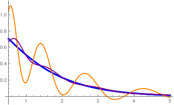
We plot a Laguerre approximations of the Bessel function with 10 terms.
bessel10[x_] = Sum[LaguerreL[n, x]/Factorial[n], {n, 0, 10}];
Laguerre approximations of the Bessel function with 10 terms.
Mathematica code.
Finally, we check validity of Paeseval's identity:
\[
2.27959 = \| F(x) \|^2 = \int_0^{\infty} \left( J_{0} \left( 2\sqrt{x} \right) \right)^2 e^{2-x} {\text d}x = \sum_{n\ge 0} \frac{1}{\left( n! \right)} .
\]
NIntegrate[(BesselJ[0, 2*Sqrt[x]]*Exp[1])^2*Exp[-x], {x, 0, 100}]
2.27959
N[Sum[1/(Factorial[n])^2 , {n, 0, 50}]]
2.27959
■
Example 7: Expansion of the trigonometric functions
Example 7:
\[
\cos x = \sum_{k\ge 0} a_{2k} L_{2k} (x) + \sum_{k\ge 0} a_{2k+1} L_{2k+1} (x) ,
\]
where coefficients are
\[
a_{n} = \int_0^{\infty} \cos x \, e^{-x} L_n (x)\,{\text d} x , \qquad n=0,1,2,\ldots .
\]
First, we perform a computational experiment.
Integrate[Cos[x]*Exp[-x]*LaguerreL[0, x], {x, 0, Infinity}]
1/2
Integrate[Cos[x]*Exp[-x]*LaguerreL[1, x], {x, 0, Infinity}]
1/2
Integrate[Cos[x]*Exp[-x]*LaguerreL[2, x], {x, 0, Infinity}]
1/4
Integrate[Cos[x]*Exp[-x]*LaguerreL[3, x], {x, 0, Infinity}]
0
Integrate[Cos[x]*Exp[-x]*LaguerreL[4, x], {x, 0, Infinity}]
-(1/8)
Integrate[Cos[x]*Exp[-x]*LaguerreL[5, x], {x, 0, Infinity}]
-(1/8)
Integrate[Cos[x]*Exp[-x]*LaguerreL[6, x], {x, 0, Infinity}]
-(1/16)
Integrate[Cos[x]*Exp[-x]*LaguerreL[7, x], {x, 0, Infinity}]
0
Integrate[Cos[x]*Exp[-x]*LaguerreL[8, x], {x, 0, Infinity}]
1/32
Integrate[Cos[x]*Exp[-x]*LaguerreL[9, x], {x, 0, Infinity}]
1/32
Integrate[Cos[x]*Exp[-x]*LaguerreL[10, x], {x, 0, Infinity}]
1/64
Therefore, we conclude that
\[
\cos x = \sum_{k\ge 0} \frac{(-1)^{
\lfloor k/2 \rfloor}}{2^{k+1}}\, L_{2k} (x) + \sum_{k\ge 0} \frac{(-1)^k}{2^{1+2k}}\, L_{4k+1} (x) .
\]
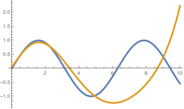
Similarly, for sine function, we get Laguerre expansion
\[
\sin x = \sum_{k\ge 0} \frac{(-1)^{
\lfloor (k+1)/2 \rfloor}}{2^{k+1}}\, L_{2k} (x) + \sum_{k\ge 0} \frac{(-1)^{k+1}}{2^{2k+2}}\, L_{4k+3} (x) .
\]
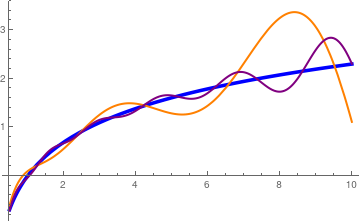
We plot these approximations
sinL10[x_] = Sum[(-1)^(Floor[(k+1)/2])*LaguerreL[2*k,x]/2^(k+1), {k,0,10}] + Sum[(-1)^(k+1)*LaguerreL[4*k+3,x]/4^(k+1), {k, 0, 10}];
Sine approximation with 10 terms.
;Sine approximation with 20 terms.
■
Example 8: Heaviside and Dirac delta function
Example 8: section ii of Tutorial I the Heaviside and Dirac delta functions.
The Laguerre expansion of the
Dirac delta function is
\[
\delta (x-a) = e^{-(x+a)/2} \,\sum_{k\ge 0} \, L_k (x) \, L_k (a) .
\]
Upon choosing a positive number
𝑎, we consider the shifted Heaviside function:
\[
H(t-a) = \begin{cases} 1, & \ \mbox{for} \quad t > a, \\
1/2, & \ \mbox{for} \quad t = a, \\
0, & \ \mbox{for} \quad t < a. \end{cases}
\]
Let us find a partial sum with
N + 1 terms of the corresponding Laguerre expansion:
\[
S_N (t) = \sum_{k=0}^N c_k L_k (t) .
\]
First, we calculate coefficients
\[
c_k = \int_a^{\infty} e^{-t} L_k (t) \,{\text d}t , \qquad k=0,1,2,\ldots .
\]
With
Mathematica , we find a few first terms:
Assuming[a > 0, Integrate[Exp[-x]*LaguerreL[0, x], {x, a, Infinity}]]
E^-a
Assuming[a > 0, Integrate[Exp[-x]*LaguerreL[1, x], {x, a, Infinity}]]
-a E^-a
Assuming[a > 0, Integrate[Exp[-x]*LaguerreL[2, x], {x, a, Infinity}]]
1/2 (-2 + a) a E^-a
Assuming[a > 0, Integrate[Exp[-x]*LaguerreL[3, x], {x, a, Infinity}]]
-(1/6) a (6 - 6 a + a^2) E^-a
Assuming[a > 0, Integrate[Exp[-x]*LaguerreL[4, x], {x, a, Infinity}]]
1/24 a (-24 + (-6 + a)^2 a) E^-a
Assuming[a > 0, Integrate[Exp[-x]*LaguerreL[5, x], {x, a, Infinity}]]
-(1/120) a (120 + a (-240 + a (120 + (-20 + a) a))) E^-a
Let us set 𝑎 = 1, we expand the shifted Heaviside function
H (
t - 1) into
Laguerre series. First, we calculate the coefficients:
Do[ c[k] = Integrate[Exp[-x]*LaguerreL[k, x], {x, 1, Infinity}], {k,
0, 10}]
Then we repeat calculations with 20 terms and 30 terms:
Do[ c[k] = Integrate[Exp[-x]*LaguerreL[k, x], {x, 1, Infinity}], {k,
11, 20}]
and
Do[ c[k] = Integrate[Exp[-x]*LaguerreL[k, x], {x, 1, Infinity}], {k,
21, 30}]
Laguerre approximation with 10 terms
Laguerre approximation with 20 terms
Laguerre approximation with 30 terms
Since finite sums exhibit Gibbs phenomenon at point x = 1, we apply Cesàro summation.
C10[x_] = Sum[c[k]*LaguerreL[k, x]*(1 -k/11), {k, 0, 10}];
Cesàro--Laguerre approximation with 10 terms
Cesàro--Laguerre approximation with 20 terms
Cesàro--Laguerre approximation with 30 terms
■
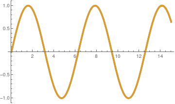
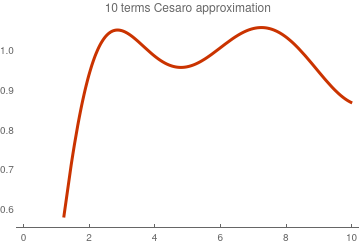
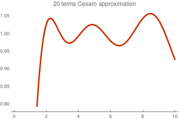
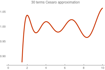
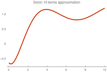
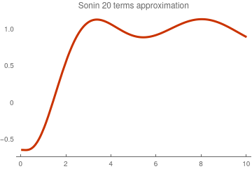
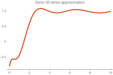
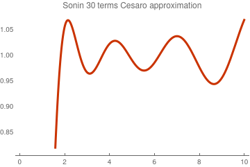
Example 9: Expansion of the signum function
Example 9:
\[
\mbox{sign}(x-a) = \begin{cases}
\phantom{-}1 , & \ a < x , \\
-1 , & \ 0 < x < a ,
\end{cases}
\]
where 𝑎 is a positive number. The Fourier coefficients are evaluated according to Eq.\eqref{EqLaguerre.8}
\[
f_k = - \frac{k!}{\Gamma (k + \alpha + 1 )} \int_0^a L_k^{(\alpha )} (x)\,x^{\alpha} e^{-x} {\text d} x + \frac{k!}{\Gamma (k + \alpha + 1 )} \int_a^{\infty} L_k^{(\alpha )} (x)\,x^{\alpha} e^{-x} {\text d} x .
\]
The signum function has the expansion:
\[
\mbox{sign}(x-a) = \sum_{k\ge 0} f_k L_k^{(\alpha )} (x) .
\]
In case of α = 0, we have
\[
\mbox{sign}(x-a) = \sum_{k\ge 0} f_k L_k (x) , \qquad f_k = -\int_0^a L_k (x) \, e^{-x} {\text d} x + \int_a^{\infty} L_k (x)\, e^{-x} {\text d} x .
\]
.
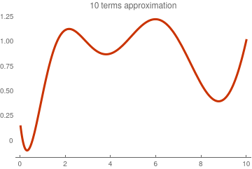
Here is Mathematica code for 𝑎 = 1 and α = ½:
Do[ f[k] = (Integrate[
Exp[-x]*LaguerreL[k, 1/2, x]*x^(1/2), {x, 1, Infinity}] -
Integrate[Exp[-x]*LaguerreL[k, 1/2, x]*x^(1/2), {x, 0, 1}])*
k! /Gamma[k + 3/2], {k, 0, 10}]
S10[x_] = Sum[f[k]*LaguerreL[k,1/2. x], {k, 0, 10}];
Plot[S10[x], {x, 0, 10}, PlotTheme -> "Web",
PlotLabel -> "Sonin 10 terms approximation"]
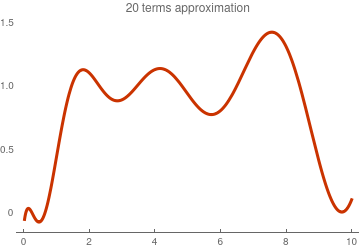
Then we repeat the calculation with 20 terms
Do[ f[k] = (Integrate[
Exp[-x]*LaguerreL[k, 1/2, x]*x^(1/2), {x, 1, Infinity}] -
Integrate[Exp[-x]*LaguerreL[k, 1/2, x]*x^(1/2), {x, 0, 1}])*
k! /Gamma[k + 3/2], {k, 11, 20}]
S20[x_] = Sum[f[k]*LaguerreL[k,1/2. x], {k, 0, 20}];
Plot[S20[x], {x, 0, 10}, PlotTheme -> "Web",
PlotLabel -> "Sonin 20 terms approximation"]
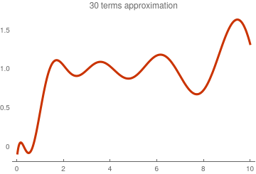
and then with 30 terms
Do[ f[k] = (Integrate[
Exp[-x]*LaguerreL[k, 1/2, x]*x^(1/2), {x, 1, Infinity}] -
Integrate[Exp[-x]*LaguerreL[k, 1/2, x]*x^(1/2), {x, 0, 1}])*
k! /Gamma[k + 3/2], {k, 21, 30}]
S30[x_] = Sum[f[k]*LaguerreL[k,1/2. x], {k, 0, 10}];
Plot[S30[x], {x, 0, 10}, PlotTheme -> "Web",
PlotLabel -> "Sonin 30 terms approximation"]
Sonin approximation with 10 terms
Sonin approximation with 20 terms
Sonin approximation with 30 terms
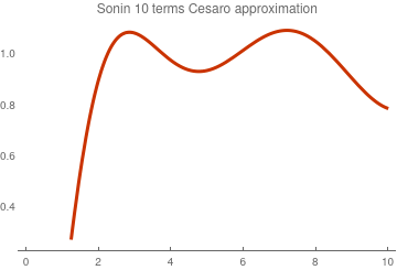
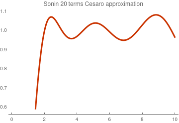
Since finite sums exhibit Gibbs phenomenon at point x = 1, we apply Cesàro summation:
\[
C_N (x) = \sum_{k=0}^N f_k L_n^{(\alpha )} (x) \left( 1 - \frac{k}{N+1} \right) .
\]
C10[x_] = Sum[f[k]*LaguerreL[k, 1/2, x]*(1 -k/11), {k, 0, 10}];
Cesàro--Sonin approximation with 10 terms
Cesàro--Sonin approximation with 20 terms
Cesàro--Sonin approximation with 30 terms
Module[{a}, coef = {};
Module[{a}, coef = {};
================================================= to be checked
Consider piecewise step function
\[
f(x) = \begin{cases}
\phantom{-}1 , & \ 0 < t < 1 , \\
-1 , & \ 1 < t .
\end{cases}
\]
Module[{a}, coef = {};
Module[{a}, coef = {};
■
Example 10: Expansion of a characteristic function
Example 10: b ]
\[
\chi_{[a,b]} (x) = \begin{cases}
1, & \ \mbox{ when} \quad a \le x \le b , \\
0, & \ \mbox{ otherwise},
\end{cases}
\]
where 0 ≤ 𝑎 <
b . Expanding this function into Fourier--Laguerre series, we get
\[
\chi_{[a,b]} (x) = \sum_{n\ge 0} c_n L_n (x) , \qquad c_n = \int_a^b L_n (x)\,e^{-x} {\text d}x .
\]
■
Connection to Hermite expansion
Suppose we know a Hermite expansion for some function
\[
\phi (x) = \sum_{n\ge 0} c_{2n} H_{2n} (x) .
\]
Using the formula
\begin{equation} \label{EqLaguerre.10}
L_n^{(\alpha )} (x) = \frac{(-1)^n \Gamma \left( n+ \alpha + 1 \right)}{(2n)! \,\sqrt{\pi}\,\Gamma \left( n + \frac{1}{2} \right)} \int_{-1}^1 \left( 1 - t^2 \right)^{\alpha - 1/2} H_{2n} \left( t\sqrt{x} \right) {\text d}t ,
\end{equation}
we get another function that we expand into Sonin series
\[
f(x) = \int_{-1}^1 \left( 1 - t^2 \right)^{\alpha - 1/2} \phi \left( t\sqrt{x} \right) {\text d}t = \sum_{n\ge 0} a_n L_n^{(\alpha )} (x) .
\]
This expansion is valid for α > −½ and its coefficients are
\[
a_n = (-1)^n \frac{\sqrt{\pi} \Gamma \left( n + \frac{1}{2} \right) (2n)!}{\Gamma \left( n+ \alpha + 1 \right)}\, c_{2n} , \qquad n=0,1,2,\ldots .
\]
Return to Mathematica page main page (APMA0340) Part 1 Matrix Algebra Part 2 Linear Systems of Ordinary Differential Equations Part 3 Non-linear Systems of Ordinary Differential Equations Part 4 Numerical Methods Part 5 Fourier Series Part 6 Partial Differential EquationsPart 7 Special Functions