Preface
This section is about application of standard Mathematica command NDSolve to the systems of ordinary differential equations.
Return to computing page for the first course APMA0330
Return to computing page for the second course APMA0340
Return to Mathematica tutorial for the first course APMA0330
Return to Mathematica tutorial for the second course APMA0340
Return to the main page for the first course APMA0330
Return to the main page for the second course APMA0340
Return to Part IV of the course APMA0340
Introduction to Linear Algebra with Mathematica
Glossary
Numerical solutions using NDSolve
The Wolfram Language function NDSolve is a general numerical differential equation solver. It can handle a wide range of ordinary differential equations (ODEs) as well as some partial differential equations (PDEs) and some differential-algebraic equations (DAEs). In a system of ordinary differential equations, there can be any number of unknown functions, but all of these functions must depend on a single independent variable, which is the same for each function.
NDSolve provides approximations to the solutions as InterpolatingFunction objects over the specified range of independent variable.
In order to get started, NDSolve has to be given appropriate initial or boundary conditions for the which the problem has a unique solution. These conditions specify values for the unknown function/solution, and perhaps its derivatives, if needed. A boundary value occurs when the unknown function is specified at multiple points. NDSolve can solve nearly all initial value problems that can symbolically be put in normal form (i.e. are solvable for the highest derivative order), but only linear boundary value problems.
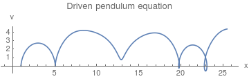
Example: Consider the driven pendulum that is modeled by the following initial value problem:
ParametricPlot[{x[t], x'[t]} /. solution, {t, 0, 14}, AxesLabel -> {"x", "v"}, PlotLabel -> "Driven pendulum equation"]
 |
 |
As mentioned earlier, NDSolve works by taking a sequence of steps in the independent variable t. NDSolve uses an adaptive procedure to determine the size of these steps. In general, if the solution appears to be varying rapidly in a particular region, then NDSolve will reduce the step size to be able to better track the solution.
NDSolve allows you to specify the precision or accuracy of result you want. In general, NDSolve makes the steps it takes smaller and smaller until the solution reached satisfies either the AccuracyGoal or the PrecisionGoal you give. The setting for AccuracyGoal effectively determines the absolute error to allow in the solution, while the setting for PrecisionGoal determines the relative error. If you need to track a solution whose value comes close to zero, then you will typically need to increase the setting for AccuracyGoal. By setting AccuracyGoal->Infinity, you tell NDSolve to use PrecisionGoal only. Generally, AccuracyGoal and PrecisionGoal are used to control the error local to a particular time step. For some differential equations, this error can accumulate, so it is possible that the precision or accuracy of the result at the end of the time interval may be much less than what you might expect from the settings of AccuracyGoal and PrecisionGoal.
NDSolve uses the setting you give for WorkingPrecision to determine the precision to use in its internal computations. If you specify large values for AccuracyGoal or PrecisionGoal, then you typically need to give a somewhat larger value for WorkingPrecision. With the default setting of Automatic, both AccuracyGoal and PrecisionGoal are equal to half of the setting for WorkingPrecision.
NDSolve uses the setting you give for WorkingPrecision to determine the precision to use in its internal computations.
NDSolve follows the general procedure of reducing step size until it tracks solutions accurately. There is a problem, however, when the true solution has a singularity. In this case, NDSolve might go on reducing the step size forever, and never terminate. To avoid this problem, the option MaxSteps specifies the maximum number of steps that NDSolve will ever take in attempting to find a solution. For ordinary differential equations, the default setting is MaxSteps->10000.
The default setting MaxSteps->10000 should be sufficient for most equations with smooth solutions. When solutions have a complicated structure, however, you may sometimes have to choose larger settings for MaxSteps. With the setting MaxSteps->Infinity there is no upper limit on the number of steps used.
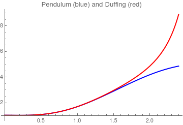
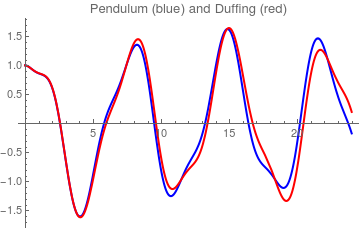
Example: The pendulum equation contains sine function depending on the angle of inclination. If we approximate this sine function by its two term Maclaurin series \( \sin x \approx x - \frac{x^3}{6} + \cdots , \) we come to the so called the Duffing equation (undamped):
WorkingPrecision option:
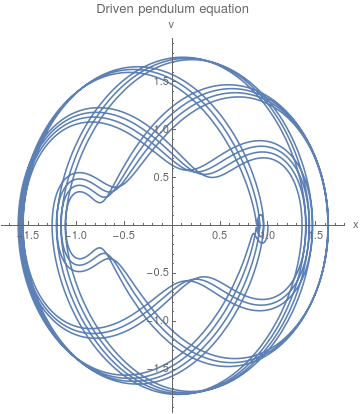
ParametricPlot[{x[t], x'[t]} /. sol150, {t, 0, 100}, AxesLabel -> {"x", "v"}, PlotLabel -> "Driven pendulum equation"]
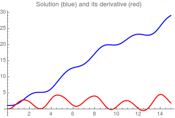
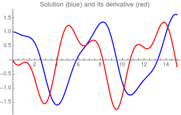
Plot[Evaluate[{x[t], x'[t]} /. sol150], {t, 0, 15}, PlotRange -> All, PlotStyle -> {{Thick, Blue}, {Thick, Red}}, PlotLabel -> "Solution (blue) and its derivative (red)" ]
 |
 |
NDSolve has several different methods built in for computing solutions as well as a mechanism for adding additional methods. With the default setting Method->Automatic, NDSolve will choose a method which should be appropriate for the differential equations. For example, if the equations have stiffness, implicit methods will be used as needed, or if the equations make a DAE, a special DAE method will be used. In general, it is not possible to determine the nature of solutions to differential equations without actually solving them: thus, the default Automatic methods are good for solving as wide variety of problems, but the one chosen may not be the best one available for your particular problem. Also, you may want to choose methods, such as symplectic integrators, which preserve certain properties of the solution.
| Order | Method | Formula |
|---|---|---|
| 1 | Explicit Euler | \( y_{n+1} = y_n + h_n f\left( x_n, y_n \right) \) |
| 2 | Explicit Midpoint | \( y_{n+1/2} = y_n + h_n \frac{1}{2} \,f\left( x_n, y_n \right) \) | \right) \)
| 1 | Backward or implicit Euler | \( y_{n+1} = y_n + h_n f\left( x_{n+1}, y_{n+1} \right) \) |
| 2 | Implicit Midpoint | \( y_{n+1} = y_n + h_n f \left( x_{n+1/2} , \frac{1}{2} \left( y_n + y_{n+1} \right) \right) \) |
| 2 | Trapezoidal | \( y_{n+1} = y_n + h_n \frac{1}{2}\, f (x_n , y_n ) + h_n \frac{1}{2}\, f \left( x_{n+1} , y_{n+1} \right) \) |
| 1 | Linearly Implicit Euler | \( \left( I - h_n J \right) \left( y_{n+1} - y_n \right) = h_n f \left( x_n , y_n ) \right) \) |
| 2 | Linearly Implicit Midpoint | \( \left( I - \frac{h_n}{2}\, J \right) \left( y_{n+1/2} - y_n \right) = \frac{h_n}{2} \, f\left( x_n , y_n \right) \)
\( \left( I - \frac{h_n}{2}\, J \right) \frac{\Delta y_n - \Delta y_{n-1/2}}{2} = \frac{h_n}{2} \,f\left( x_{n+1/2}, y_{n+1/2} \right) - \Delta y_{n-1/2} \) |
When NDSolve computes a solution, there are typically three phases. First, the equations are processed, usually into a function that represents the right-hand side of the equations in normal form. Next, the function is used to iterate the solution from the initial conditions. Finally, data saved during the iteration procedure is processed into one or more InterpolatingFunction objects. Using functions in the NDSolve` context, you can run these steps separately and, more importantly, have more control over the iteration process. The steps are tied by an NDSolve`StateData object, which keeps all of the data necessary for solving the differential equations.
Return to Mathematica page
Return to the main page (APMA0340)
Return to the Part 1 Matrix Algebra
Return to the Part 2 Linear Systems of Ordinary Differential Equations
Return to the Part 3 Non-linear Systems of Ordinary Differential Equations
Return to the Part 4 Numerical Methods
Return to the Part 5 Fourier Series
Return to the Part 6 Partial Differential Equations
Return to the Part 7 Special Functions