The
Laplace transfrom is an integral transformation that maps a function
f (
t ) of a real variable
t ∈ [0, ∞) into a number depending on parameter λ:
\begin{equation} \label{EqLaplace.1}
{\cal L} \left[ f(t) \right] (\lambda ) = f^L (\lambda ) = \int_0^{\infty} f(t)\, e^{-\lambda t} {\text d} t ,
\end{equation}
subject that the integral converges. Since we are going to apply the Laplace transformation for solving differential equations, it will be always assumed that the unknown function and all its derivatived that appear in the differential equation possess convergent Laplace transforms. Since this topic was explored previously in the first
tutorial , we omit repeating properties of the Laplace transform and corresponding historical notes. A reader who needs to recollect more details about the Laplace transform, it recommended to return to the mentioned tutorial for the first course.
The main reason why the Laplace transform is a successful tool for solving differential equations is that it provides the spectral decomposition to the derivative operator, that is,
\begin{equation} \label{EqLaplace.2}
{\cal L} \left[ \texttt{D}f(t) \right] (\lambda ) = \lambda \,f^L (\lambda ) - f(+0) = \lambda\,{\cal L} \left[ f(t) \right] (\lambda ) - f(+0), \qquad \texttt{D} = \frac{\text d}{{\text d}t} ,
\end{equation}
acting on the space of the smooth functions defined on the positive half-line ℝ
+ = [0, ∞). Therefore, the Laplace transform works well for differential equations with constant coefficients, not necessary written in normal form. The advantage of the Laplace transformation becomes clear when it is applied to inhomogeneous equations, especially with piecewise continuous input functions. We demonstrate its approach in numerous examples.
The reader should remember that the inverse Laplace transform is an ill-posed problem . However, in applications of the Laplace transformations to ordinary differential equations (ODEs), the inverse Laplace transform can be obtained using the residue theorem:
\begin{equation} \label{EqLaplace.3}
f(t) = {\cal L}^{-1} \left[ f^L (\lambda ) \right] (t ) =
\left[ \sum_k \mbox{Res}_{\lambda_k} \, f^L (\lambda )\, e^{\lambda\,t} \right] H(t) ,
\end{equation}
where summation is expanded over all singular points (poles) of the function
f L and
H (
t ) is the
Heaviside function .
Application of the Laplace transform for linear systems of first order differential equations in normal form is straight forward. Consider the initial value problem for the homogeneous equation:
\begin{equation} \label{EqLaplace.4}
\frac{\text d}{{\text d}t} \,{\bf x} = {\bf A}\,{\bf x}(t) , \qquad {\bf x}(0) = {\bf x}_0 ,
\end{equation}
where
A is a constant square matrix and
x (
t ) is a column vector of unknown functions. Application of the Laplace transform to the IVP yields
\[
\lambda\,{\bf x}^L = {\bf A}\,{\bf x}^L + {\bf x}_0 \qquad \Longrightarrow \qquad {\bf x}^L = \left( \lambda\,{\bf I} - {\bf A} \right)^{-1} {\bf x}_0 = {\bf R}_{\lambda} ({\bf A})\, {\bf x}_0 ,
\]
where
\[
{\bf R}_{\lambda} ({\bf A}) = \left( \lambda\,{\bf I} - {\bf A} \right)^{-1}
\]
is the resolvent of the matrix
A . Applying the inverse Laplace transform, we obtain
\[
{\bf x}(t) = {\cal L}^{-1} \left[ {\bf R}_{\lambda} ({\bf A}) \, {\bf x}_0 \right] = {\cal L}^{-1} \left[ \left( \lambda\,{\bf I} - {\bf A} \right)^{-1} \, {\bf x}_0 \right] = e^{{\bf A}\,t} {\bf x}_0 .
\]
So the resolvent of a square matrix is the Laplace transform of the
exponential matrix. For further applications of the Laplace transformation, we recommend to visit two other sections:
second order systems and
spring-mass systems .
Example 1: 2×2 homogeneous system
Example 1:
Consider the planar homogeneous system of differential equations
\[
\frac{\text d}{{\text d}t} \begin{bmatrix} x(t) \\ y(t) \end{bmatrix} = {\bf A} \begin{bmatrix} x(t) \\ y(t) \end{bmatrix} , \qquad \begin{bmatrix} x(0) \\ y(0) \end{bmatrix} = \begin{bmatrix} \phantom{-}2 \\ -1 \end{bmatrix} , \qquad {\bf A} =
\begin{bmatrix} 1&3 \\ 4&2 \end{bmatrix} .
\]
DSolve[{x'[t] == x[t] + 3*y[t], y'[t] == 4*x[t] + 2*y[t], x[0] == 2,
y[0] == -1}, {x[t], y[t]}, t]
{{x[t] -> 1/7 E^(-2 t) (11 + 3 E^(7 t)),
y[t] -> 1/7 E^(-2 t) (-11 + 4 E^(7 t))}}
\[
x(t) = \frac{1}{7} \left( 11\,e^{-2t} + 3\, e^{5t} \right) , \qquad y(t) = \frac{1}{7} \left( -11\,e^{-2t} + 4\, e^{5t} \right)
\]
■
Example 2: 2×2 homogeneous system not in normal form
Example 2:
Recall that a system of equations is referred to be in normal form if the highest derivatives are isolated and each such derivative is of the same order. Now we consider the planar system
\[
\begin{cases}
x' + 2\,y' + x + 3\,y &=0,
\\
3\,x' + 4\,y' -x + 6\,y &= 0,
\end{cases} \qquad x(0) = 2, \quad y(0) = -1.
\]
Of course,
Mathematica is capable to solve such kind of equations.
DSolve[{x'[t] + 2*y'[t] + x[t] + 3*y[t] == 0,
3*x'[t] + 4*y'[t] - 1*x[t] + 6 y[t] == 0, x[0] == 2,
y[0] == -1}, {x[t], y[t]}, t]
{{x[t] -> 2 E^(3 t), y[t] -> -(1/9) E^(-3 t/2) (1 + 8 E^(9 t/2))}}
\[
x(t) = 2\,e^{3t} H(t) , \qquad y(t) = -\frac{1}{9} \left( e^{-3t/2} + 8\,e^{3t} \right) H(t) ,
\]
where
H (
t ) is the
Heaviside function .
Nevertheless, we demonstrate the effectiveness of the Laplace transformation technique in this case. Application of the Laplace transform to the given system of differential equations yields
\[
\begin{split}
\lambda \,x^L + 2\lambda\,y^L + x^L + 3\,y^L &= x(0) + 2 y(0),
\\
3\lambda\,x^L + 4\lambda\,y^L -x^L + 6\,y^L &= 3x(0) + 4y(0),
\end{split}
\tag{2.1}
\]
where
\[
x^L = \int_0^{\infty} e^{-\lambda t}x(t) \,{\text d}t \qquad\mbox{and} \qquad
y^L = \int_0^{\infty} e^{-\lambda t}y(t) \,{\text d}
\]
are Laplace transforms of unknown functions
x (
t ) and
y (
t ), respectively. We solve the system of algebraic equations (3.1) with the aid of
Mathematica :
Solve[{(s + 1)*x + (2*s + 3)*y == 0, (3*s - 1)*x + (4*s + 6)*y ==
2}, {x, y}]
{{x -> 2/(-3 + s), y -> -((2 (1 + s))/((-3 + s) (3 + 2 s)))}}
\[
x^L = \frac{2}{3+\lambda} , \qquad y^L = \frac{2 \left( 1+\lambda \right)}{\left( \lambda -3 \right)\left( 2\lambda +3 \right)} .
\]
Applying the inverse Laplace transform, we obtain the required solutions.
InverseLaplaceTransform[%, s, t]
End of Example 2
■
The nonhomogeneous systems
\begin{equation} \label{EqLaplace.5}
\frac{\text d}{{\text d}t} \,{\bf x} = {\bf A}\,{\bf x}(t) + {\bf f}(t), \qquad {\bf x}(0) = {\bf x}_0 ,
\end{equation}
can be solved similarly. Using the Laplace transform, we get
\[
\lambda\,{\bf x}^L = {\bf A}\,{\bf x}^L + {\bf x}_0 + {\bf f}^L \qquad \Longrightarrow \qquad {\bf x}^L = \left( \lambda\,{\bf I} - {\bf A} \right)^{-1} {\bf x}_0 + {\bf R}_{\lambda} ({\bf A})\, {\bf f}^L ,
\]
where
f L is the Laplace transform of the forcing function. This gives
\begin{equation} \label{EqLaplace.6}
{\bf x} (t) = {\cal L}^{-1} \left[ \left( \lambda\,{\bf I} - {\bf A} \right)^{-1} {\bf x}_0 \right] + {\cal L}^{-1} \left[ \left( \lambda\,{\bf I} - {\bf A} \right)^{-1} {\bf f}^L \right] .
\end{equation}
Again, application of the inverse Laplace transform yields the well-known formula for the required solution:
\begin{equation} \label{EqLaplace.7}
{\bf x} (t) = e^{{\bf A}\,t} {\bf x}_0 + \int_0^t e^{{\bf A}\,(t- \tau )} {\bf f}(\tau ) \,{\text d} \tau .
\end{equation}
The main advantage of the Laplace transformation compared to other methods is observed in systems with piecewise continuous inputs.
Example 3: 2×2 inhomogeneous system
Example 3:
Consider the planar system
\[
\begin{split}
\dot{x} &= 3x(t) -2\,y(t) + e^{-t} \cos 3t ,
\\
\dot{y} &= 2\,x(t) - y(t) ,
\end{split} \qquad
\begin{split} x(0) = -1 , \\ y(0) = \phantom{-}1 . \end{split}
\tag{1.1}
\]
It is convenient to rewrite the given problem in vector form:
\[
\frac{\text d}{{\text d}t} \begin{bmatrix} x(t) \\ y(t) \end{bmatrix} = \begin{bmatrix} 3&-2 \\ 2&-1 \end{bmatrix} \begin{bmatrix} x(t) \\ y(t) \end{bmatrix} + \begin{bmatrix} e^{-t} \cos 3t \\ 0 \end{bmatrix} .
\tag{1.2}
\]
So using the following notation
\[
{\bf x} (t) = \begin{bmatrix} x(t) \\ y(t) \end{bmatrix} , \qquad {\bf A} = \begin{bmatrix} 3&-2 \\ 2&-1 \end{bmatrix} , \qquad {\bf f}(t) = \begin{bmatrix} e^{-t} \cos 3t \\ 0 \end{bmatrix} , \qquad {\bf x}_0 = \begin{bmatrix} -1 \\ \phantom{-}1 \end{bmatrix} ,
\]
we rewrite \Eq(1.2) in concise form:
\[
\dot{\bf x} (t) = {\bf A}\,{\bf x}(t) + {\bf f}(t) , \qquad {\bf x}(0) = {\bf x}_0 .
\tag{1.3}
\]
Taking the Laplace transform of the system (1.3) gives
\[
\lambda \,{\bf x}^L = {\bf A}\,{\bf x}^L + {\bf x}_0 + {\bf f}^L ,
\]
where
\[
{\bf x}^L = {\cal L} \left[ {\bf x}(t) \right] = \int_0^{\infty} e^{-\lambda t} {\bf x}(t) \,{\text d}t = \begin{bmatrix} x^L \\ y^L \end{bmatrix} , \qquad
{\bf f}^L = \int_0^{\infty} e^{-\lambda t} {\bf f}(t) \,{\text d}t = \begin{bmatrix} \frac{1 + \lambda}{9 + (1+\lambda )^2} \\ 0 \end{bmatrix}
\]
LaplaceTransform[Exp[-t]*Cos[3*t], t, s]
(1 + s)/(9 + (1 + s)^2)
Since the resolvent of the matrix
A is
\[
{\bf R}_{\lambda} ({\bf A}) = \left( \lambda {\bf I} - {\bf A} \right)^{-1} = \frac{1}{(\lambda - 1)^2} \begin{bmatrix} 1 + \lambda & -2 \\ 2 & \lambda -3 \end{bmatrix} ,
\]
Inverse[s*IdentityMatrix[2] - {{3, -2}, {2, -1}}]
{{(1 + s)/(1 - 2 s + s^2), -(2/(1 - 2 s + s^2))}, {2/(
1 - 2 s + s^2), (-3 + s)/(1 - 2 s + s^2)}}
we get the Laplace transform of the solution to be
\[
{\bf x}^L = \frac{1}{(\lambda - 1)^2} \begin{bmatrix} 1 + \lambda & -2 \\ 2 & \lambda -3 \end{bmatrix} \begin{bmatrix} -1 \\ \phantom{-}1 \end{bmatrix} + \frac{1}{(\lambda - 1)^2} \begin{bmatrix} 1 + \lambda & -2 \\ 2 & \lambda -3 \end{bmatrix} \frac{1}{9 + (1 + \lambda )^2} \begin{bmatrix} 1 + \lambda \\ 0 \end{bmatrix} .
\]
In other words,
\[
{\bf x}^L = \frac{1}{(\lambda - 1)^2} \begin{bmatrix} -\lambda -3 \\ \lambda -5 \end{bmatrix} + \frac{1}{(\lambda - 1)^2}\cdot \frac{1}{9 + (1 + \lambda )^2} \begin{bmatrix} (\lambda + 1)^2 \\ 2(1+\lambda ) \end{bmatrix} .
\tag{1.4}
\]
To find the solution, we just need to apply the inverse Laplace transform. First, we use
Mathematica to determine components of the solution:
\begin{align*}
{\cal L}^{-1} \left[ \frac{1}{(\lambda - 1)^2} \right] &= t\, e^t ,
\\
{\cal L}^{-1} \left[ \frac{\lambda}{(\lambda - 1)^2} \right] &= e^t \left( 1 - t \right) ,
\\
{\cal L}^{-1} \left[ \frac{\lambda +1}{(\lambda - 1)^2} \cdot \frac{1}{9 + (1 + \lambda )^2}\right] &= \frac{5 + 26t}{169}\,e^t - \frac{1}{169}\, e^{-t} \left[ 5\,\cos 3t + 12\,\sin 3t \right] ,
\\
{\cal L}^{-1} \left[ \frac{(\lambda +1)^2}{(\lambda - 1)^2} \cdot \frac{1}{9 + (1 + \lambda )^2}\right] &= \frac{4 \left( 9 - 13t \right)}{169}\, e^t + \frac{1}{169}\, e^{-t} \left[ 15\,\sin 3t - 36\,\cos 3t \right] .
\end{align*}
InverseLaplaceTransform[1/(s - 1)^2, s, t]
E^t t
InverseLaplaceTransform[s/(s - 1)^2, s, t]
E^t (1 + t)
InverseLaplaceTransform[(s + 1)/(s - 1)^2/(9 + (1 + s)^2), s, t]
1/169 E^-t (E^(2 t) (5 + 26 t) - 5 Cos[3 t] - 12 Sin[3 t])
InverseLaplaceTransform[(s + 1)^2/(s - 1)^2/(9 + (1 + s)^2), s, t]
1/338 E^-t (8 E^(2 t) (9 + 13 t) - 72 Cos[3 t] + 30 Sin[3 t])
■
Example 4: Discontinuous input
Example 4:
We reconsider the previous differential equation, but now with discontinuous input function:
\[
\begin{split}
\dot{x} &= 3x(t) -2\,y(t) + \cos 3t \,H(t-\pi ),
\\
\dot{y} &= 2\,x(t) - y(t) + (t-1)\left[ H(t-1) - H(t-2) \right] .
\end{split}
\]
■
Example 5: Three-loop electric circuit
Example 5:
We have already considered circuits in our
motivating section and the first
tutorial . There are several reasons for this, among them the importance of circuit theory and the pervasiveness of differential equations in circuit theory.
Recall that the word circuit means that quantities such as current are determined solely by position along the path. We ignore field effects that occur in wires connecting electric elements. We consider only lumped-parameter circuits, which means that the effects of the various electrical components may be considered to be concentrated at one point. At each point in the circuit there are two quantities of interest: voltage (or potential) and current (or net flow of positive charges). A branch is part of a circuit where two terminals to which connections can be made, a node is a point where two or more branches come together, and a loop is a closed path formed by connecting branches.
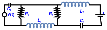
Although most electric circuits include multiple loops, we consider only three-loop circuits of the general form:
coil2 = ParametricPlot[{1*Cos[t*3 + Pi] + 1.5*t + 22.5,
2*Sin[t*3] + 11.5}, {t, 0, 5*Pi}, Ticks -> None, Axes -> False,
ImageSize -> Tiny, PlotStyle -> {Thickness[0.01]}];
Three-loop circuit.
We apply the Kirchhoff voltage law to every loop. So for the left loop, we have
\[
\frac{1}{C_1}\, q_1 + R_1 i_1 = v(t) ,
\]
where
q 1 (
t ) is the charge in the capacitor and
i 1 (
t ) = d
q 1 /d
t is the current in the first loop, which is the derivative of the charge.
For the middle loop, we have
\[
R_1 \left( i_1 - i_2 \right) + R_2 \left( i_2 - i_3 \right) + L_1 \frac{{\text d}i_2}{{\text d}t} = 0 .
\]
Similarly for the right loop, we get
\[
L_2 \frac{{\text d}i_3}{{\text d}t} + \frac{1}{C_2}\,q_3 + R_3 \left( i_3 - i_2 \right) = e_3 (t) ,
\]
where
e 3 is the voltage provided by the battery. We assume that
\[
e(t) = E_0 \cos \left( \omega t \right) \left[ H(t) - H(t-5) \right] , \qquad e_3 (t) = 6 \left[ H(t) - H(t-5) \right] ,
\]
where ω = 120π and
H (
t ) is the
Heaviside function :
\[
H(t) = \begin{cases}
1, & \ \mbox{when} \quad t > 0 , \\
1/2 , & \ \mbox{for } t=0, \\
0, & \ \mbox{when} \quad t < 0 .
\end{cases}
\]
Adding the relation between charge and current, we get six equations with six unknowns:
\[
i_1 = \frac{{\text d}q_1}{{\text d}t} , \qquad i_2 = \frac{{\text d}q_2}{{\text d}t} , \qquad i_3 = \frac{{\text d}q_3}{{\text d}t} .
\]
Assuming homogeneous initial conditions, we obtain upon application of the Laplace transform that
\begin{align*}
\frac{1}{C_1}\, q^L_1 + R_1 i^L_1 &= v^L = e^{-\lambda}\frac{\lambda \cos \omega - \omega \sin 5 \omega}{\lambda^2 + \omega^2} - e^{-5\lambda} \frac{\lambda \cos 5 \omega}{\lambda^2 + \omega^2} + \frac{\omega \sin 5 \omega}{\lambda^2 + \omega^2},
\\
R_1 \left( i^L_1 - i^L_2 \right) + R_2 \left( i^L_2 - i^L_3 \right) + L_1 \lambda \,i^L_2 &= 0 ,
\\
L_2 \lambda \,i^L_3 + \frac{1}{C_2}\,q^L_3 + R_3 \left( i^L_3 - i^L_2 \right) &= e^L_3 = \frac{6}{\lambda} \left( e^{-\lambda} - e^{-5\lambda} \right) ,
\end{align*}
Integrate[Cos[omega*t]*Exp[-s*t], {t, 1, 5}]
(E^(-5 s) (-s Cos[5 omega] +
E^(4 s) (s Cos[omega] - omega Sin[omega]) +
omega Sin[5 omega]))/(omega^2 + s^2)
Integrate[Exp[-s*t], {t, 1, 5}]
(E^(-5 s) (-1 + E^(4 s)))/s
and
\[
i_1^L = \lambda q_1^L , \qquad i_2^L = \lambda q_2^L , \qquad i_3^L = \lambda q_3^L .
\]
When we set ω = 120π, we get
\[
v^L = \frac{\lambda}{\lambda^2 + \omega^2} \left( e^{-\lambda} - e^{-5\lambda} \right) .
\]
% /. omega -> 120*Pi
(E^(-5 s) (-s + E^(4 s) s))/(14400 \[Pi]^2 + s^2)
Now we solve the system of algebraic equations with Mathematica :
Solve[{q1/C1 + s*R1*q1 == e1,
R1*s*(q1 - q2) + R1*s*(q2 - q3) + L1*s^2*q2 == 0,
L2*s^2 *q3 + q3/C2 + R2*s (q3 - q2) == e3}, {q1, q2, q3}]
{{q1 -> (C1 e1)/(1 + C1 R1 s),
q2 -> (-C1 e1 R1 + C2 e3 R1 + C1 C2 e3 R1^2 s - C1 C2 e1 R1 R3 s -
C1 C2 e1 L2 R1 s^2)/(
s (1 + C1 R1 s) (L1 - C2 R1 R3 + C2 L1 R2 s + C2 L1 L2 s^2)),
q3 -> (C2 (-e3 L1 + C1 e1 R1 R2 - C1 e3 L1 R1 s))/((1 +
C1 R1 s) (-L1 + C2 R1 R2 - C2 L1 R2 s - C2 L1 L2 s^2))}}
\[
q_1^L = \frac{C_1}{1 + \lambda C_1 R_1}\, v^L ,
\]
\[
q_2^L = -\frac{C_1 R_1 + C_1 C_2 R_1 R_2 \lambda +C_1 C_2 L_2 R_1 \lambda^2}{\lambda \left( 1 + C_1 R_1 \lambda \right) \left( L_1 -C_2 R_1 R_3 + C_2 L_1 R_3 \lambda + C_2 L_1 L_2 \lambda^2 \right)}\, v^L + \frac{C_2 R_1 - C_1 C_2 R_1^2 \lambda}{\lambda \left( 1 + C_1 R_1 \lambda \right) \left( L_1 -C_2 R_1 R_2 + C_2 L_1 R_2 \lambda + C_2 L_1 L_2 \lambda^2 \right)} \, \frac{6}{\lambda} \left( e^{-\lambda} - e^{-5\lambda} \right) ,
\]
and
\[
q_3^L = \frac{C_1 R_1 R_2}{\left( 1 + C_1 R_1 \lambda \right)\left( C_2 R_1 R_2 -L_1 -C_2 L_1 R_2 \lambda - C_2 L_1 L_2 \lambda^2 \right)}\, v^L - \frac{C_2 L_1 + C_1 L_1 R_1 \lambda}{\left( 1 + C_1 R_1 \lambda \right)\left( C_2 R_1 R_2 -L_1 -C_2 L_1 R_2 \lambda - C_2 L_1 L_2 \lambda^2 \right)} \, \frac{6}{\lambda} \left( e^{-\lambda} - e^{-5\lambda} \right) ,
\]
Since these expressions are very combersome, we set some numberical values:
\[
C_1 = 1, \quad L_2 = 2, \quad R_1 = 3, \quad R_2 = 4, \quad L_1 = 5, \quad C_2 = 6.
\]
Wi this in hand, we solve the corresponding system of algebraic equations for unknown Laplace transforms of three charges:
Solve[{q1 + s*3*q1 == e1,
3*s*(q1 - q2) + 3*s*(q2 - q3) + 5*s^2*q2 == 0,
2*s^2 *q3 + q3/6 + 4*s (q3 - q2) == e3}, {q1, q2, q3}]
{{q1 -> e1/(1 + 3 s),
q2 -> (3 (-e1 + 6 e3 - 24 e1 s + 18 e3 s - 12 e1 s^2))/(
s (1 + 3 s) (-67 + 120 s + 60 s^2)),
q3 -> (6 (-12 e1 + 5 e3 + 15 e3 s))/((1 + 3 s) (-67 + 120 s +
60 s^2))}}
\[
q_1^L = \frac{1}{1 + 3\lambda}\, v^L ,
\]
\[
q_2^L = -3\,\frac{1 + 24\lambda + 12 \lambda^2}{\lambda \left( 1 + 3\lambda \right)\left( 60 \lambda^2 + 120 \lambda -67 \right)} \, v^L + 3\,\frac{6 -18\lambda}{\lambda \left( 1 + 3\lambda \right)\left( 60 \lambda^2 + 120 \lambda -67 \right)} \, \frac{6}{\lambda} \left( e^{-\lambda} - e^{-5\lambda} \right) ,
\]
and
\[
q_3^L = -6\, \frac{12}{\left( 1 + 3\lambda \right)\left( 60 \lambda^2 + 120 \lambda -67 \right)} \,v^L + 6\, \frac{5 + 15 \lambda}{\left( 1 + 3\lambda \right)\left( 60 \lambda^2 + 120 \lambda -67 \right)} \, \frac{6}{\lambda} \left( e^{-\lambda} - e^{-5\lambda} \right) .
\]
Finally, we find the inverse Laplace transform of each component and then add them together. To determine
q 1 (
t ), we need only two components:
\[
g_{11} (t) = {\cal L}^{-1} \left[ \frac{1}{1 + 3\lambda}\,\frac{\lambda}{\lambda^2 + \omega^2} \right] = \left[ \frac{\cos \omega t -3\omega\,\sin \omega t}{1 + 9\omega^2} - \frac{e^{-t/3}}{1 + 9\omega^2} \right] H(t) ,
\]
\[
g_{12} (t) = {\cal L}^{-1} \left[ \frac{1}{1 + 3\lambda}\,\frac{1}{\lambda^2 + \omega^2} \right] = \left[ \frac{3\,e^{-t/3}}{1 + 9\omega^2} - \frac{3\omega\,\cos \omega t- \sin \omega t}{1 + 9\omega^2} \right] H(t) .
\]
InverseLaplaceTransform[s/(1 + 3*s)/(s^2 + omega^2), s, t]
-(E^(-t/3)/(1 + 9 omega^2)) + (Cos[omega t] + 3 omega Sin[omega t])/(
1 + 9 omega^2)
InverseLaplaceTransform[1/(1 + 3*s)/(s^2 + omega^2), s, t]
(3 E^(-t/3))/(
1 + 9 omega^2) + (-3 omega Cos[omega t] + Sin[omega t])/(
omega (1 + 9 omega^2))
Then the charge in the firs loop becomes
\[
q_1 (t) = g_{11} (t-1) \,\cos \omega - \omega\,\sin 5\omega \,g_{12} (t-1) -\cos 5\omega\,g_{11} (t-5) + \omega \sin 5\omega \,g_{12} (t-5) .
\]
Using numerical value ω = 120π, we simplify the latter:
\[
q_1 (t) = g_{11} (t-1) - g_{11} (t-5) .
\]
To determine q 2 (t ), we need another two auxiliary functions:
\begin{align*}
g_{21} (t) &= {\cal L}^{-1} \left[ -3\,\frac{1 + 24\lambda + 12 \lambda^2}{\lambda \left( 1 + 3\lambda \right)\left( 60 \lambda^2 + 120 \lambda -67 \right)} \,\frac{\lambda}{\lambda^2 + \omega^2} \right]
\\
&=
\\
g_{22} (t) &= {\cal L}^{-1} \left[ 3\,\frac{6 -18\lambda}{\lambda \left( 1 + 3\lambda \right)\left( 60 \lambda^2 + 120 \lambda -67 \right)} \, \frac{6}{\lambda} \right]
\\
&=
\end{align*}
Then
\[
q_2 (t) = g_{21} (t-1) - g_{21} (t-5) + g_{22} (t-1) - g_{22} (t-5) .
\]
Finally, we determine two auxiliary functions for the charge in the third loop:
\begin{align*}
g_{31} (t) &= {\cal L}^{-1} \left[ -6\, \frac{12}{\left( 1 + 3\lambda \right)\left( 60 \lambda^2 + 120 \lambda -67 \right)} \,\frac{\lambda}{\lambda^2 + \omega^2} \right]
\\
&=
\\
g_{32} (t) &= {\cal L}^{-1} \left[ \frac{5 + 15 \lambda}{\left( 1 + 3\lambda \right)\left( 60 \lambda^2 + 120 \lambda -67 \right)} \, \frac{36}{\lambda} \right]
\\
&=
\end{align*}
Then
\[
q_3 (t) = g_{31} (t-1) - g_{31} (t-5) + g_{32} (t-1) - g_{32} (t-5) .
\]
We can find the currents in each loop by differentiating the formulas for corresponding charges.
■
Although homogeneous differential equations of arbitrary order in normal form with constant coefficients can be solved in straightforward matter by converting them into system of first order ODEs, we demonstrate that this is not necessarily. So we start with a homogeneous system of equations in normal form
\begin{equation} \label{EqLaplace.8}
\ddot{\bf x} + {\bf B}\dot{\bf x} + {\bf A}\,{\bf x} = {\bf 0} , \qquad {\bf x} (0) = {\bf d} , \quad \dot{\bf x} (0) = {\bf v} ,
\end{equation}
where dot stands for the derivative with respect to time variable,
x (
t ) is a column-vector of unknown functions and
A and
B are constant
n ×
n matrices. Here
0 is
n column zero vector, and
d and
v are initial (known) displacements and velocity vectors.
Application of the Laplace transformation to the given initial value problem \eqref{EqLaplace.8} yields the algebraic vector equation
\[
\left( \lambda^2 {\bf I} + \lambda {\bf B} + {\bf A} \right) {\bf x}^L = {\bf v} + \lambda {\bf d} + {\bf B} {\bf d} ,
\]
with respect to the Laplace transform of the unknown vector:
\[
{\bf x}^L (\lambda ) = \int_0^{\infty} e^{-\lambda t} {\bf x}(t)\,{\text d}t .
\]
It is not hard to solve the algebraic system of equations:
\[
{\bf x}^L = \left( \lambda^2 {\bf I} + \lambda {\bf B} + {\bf A} \right)^{-1} \left( {\bf v} + \lambda {\bf d} + {\bf B} {\bf d} \right) .
\]
Applying the inverse Laplace transform, we obtain the required solution:
\begin{equation} \label{EqLaplace.9}
{\bf x}(t) = {\cal L}^{-1} \left[ \left( \lambda^2 {\bf I} + \lambda {\bf B} + {\bf A} \right)^{-1} \left( \lambda {\bf I} + {\bf B} \right) \right] {\bf d} + {\cal L}^{-1} \left[ \left( \lambda^2 {\bf I} + \lambda {\bf B} + {\bf A} \right)^{-1} \right] {\bf v} .
\end{equation}
where ℒ
-1 denotes the inverse Laplace transform. When matrix
B is zero matrix, we get a familiar formula:
\begin{equation} \label{EqLaplace.10}
{\bf x}(t) = {\cal L}^{-1} \left[ \left( \lambda^2 {\bf I} + {\bf A} \right)^{-1} \lambda \right] {\bf d} + {\cal L}^{-1} \left[ \left( \lambda^2 {\bf I} + {\bf A} \right)^{-1} \right] {\bf v} =
\cos \left( \sqrt{\bf A} t \right) {\bf d} + \frac{\sin \left( \sqrt{\bf A} t \right) }{\sqrt{\bf A}}\.{\bf v} .
\end{equation}
Example 6: Second order homogeneous system of equations
Example 6:
Example 7: Spring-mass system with viscous damping
Example 7:
The initial values problems for inhomogeneous differential vector equations can be solved with the aid of the Laplace transform in straight forward manner.
\begin{equation} \label{EqLaplace.11}
\ddot{\bf x} + {\bf B}\dot{\bf x} + {\bf A}\,{\bf x} = {\bf f} , \qquad {\bf x} (0) = {\bf d} , \quad \dot{\bf x} (0) = {\bf v} ,
\end{equation}
where
f (
t ) is the given input vector (forcing functions).
We give some examples with paying attention to intermittent forcing functions.
Example 8: Second order homogeneous with continuous input
Example 8:
Consider the initial value problem (IVP):
\[
\begin{split}
\dot{x} &= \phantom{-}2\,x - y + 3\,e^{2t} ,
\\
\dot{y} &= -2\,x + 3\,y - 5\,e^{-t} ,
\end{split} \qquad x(0) = 2, \quad y(0) = -1.
\]
■
Example 9: Second order inhomogeneous with intermittent forcing function
Example 9:
Consider the initial value problem
\[
\begin{split}
\dot{x} &= \phantom{-}2\,x - y + t \left[ H(t-\pi ) - H(t-5\pi ) \right] ,
\\
\dot{y} &= -2\,x + 3\,y - 3\,\sin t \left[ H(t-\pi ) - H(t-5\pi ) \right] ,
\end{split} \qquad x(0) = 2, \quad y(0) = -1.
\]
■
Example 10: Spring-mass system with piecewise input
Example 10:
For simplicity, we consider only planar systems of the form
\begin{equation} \label{EqLaplace.12}
\begin{split}
L_{11} \left[ \texttt{D} \right] x(t) + L_{12} \left[ \texttt{D} \right] y(t) &= f(t) , \\
L_{21} \left[ \texttt{D} \right] x(t) + L_{22} \left[ \texttt{D} \right] y(t) &= g(t) ,
\end{split}
\end{equation}
where
\[
L_{11} \left[ \texttt{D} \right] = a_2 \texttt{D}^2 + a_1 \texttt{D} + a_0 \texttt{D}^0 , \qquad L_{12} \left[ \texttt{D} \right] = b_2 \texttt{D}^2 + b_1 \texttt{D} + b_0 \texttt{D}^0 ,
\]
and
\[
L_{21} \left[ \texttt{D} \right] = c_2 \texttt{D}^2 + c_1 \texttt{D} + c_0 \texttt{D}^0 , \qquad L_{22} \left[ \texttt{D} \right] = d_2 \texttt{D}^2 + d_1 \texttt{D} + d_0 \texttt{D}^0 ,
\]
are linear differential operators with constant coefficients; as usual, we denote by
\( \texttt{D} = {\text d}/{\text d}t \) the derivative operator with respect to time variable
t with understanding that
\( \texttt{D}^0 = \texttt{I} \) is the identity operator.
The differential operator
\[
W \left[ \texttt{D} \right] = \det \begin{pmatrix} L_{11} \left[ \texttt{D} \right] & L_{12} \left[ \texttt{D} \right] \\ L_{21} \left[ \texttt{D} \right] & L_{22} \left[ \texttt{D} \right]
\end{pmatrix} = L_{11} \,L_{22} - L_{12} \,L_{21}
\]
is called the
Wronskian determinant or operational determinant of differential operators
L 11 ,
L 12 ,
L 21 , and
L 22 . If the Wronskian is identically zero, then then the system \eqref{EqLaplace.12} is said to be
degenerate .
We consider application of the Laplace transformation only to not degenerate systems having the Wronskian as an operator of order
four .
Theorem: \( \texttt{D} \) is the number of arbitrary constants in the general solution of Eq.\eqref{EqLaplace.12}, which is the number of required initial conditions needed to obtain the unique solution.
Example 11: Three derivatives, two arbitrary constants
Example 11:
Consider the linear system of differential equations with constant coefficients
\[
\begin{split}
\ddot{x}(t) + \dot{y}(t) -3\,x(t) + 5y(t) &= 2,
\\
3\ddot{x}(t) + 3\dot{y}(t) -7\,x(t) + 2\,y(t) &=t .
\end{split}
\]
Since this system involves second derivative of
x (
t ) and first derivative of
y (
t ), one might expect the answer to involve three arbitrary constants. The Wronskian corresponding to the given system is
\[
W \left[ \texttt{D} \right] = \det \begin{pmatrix} \texttt{D}^2 -3 & \texttt{D} + 5 \\ 3\texttt{D} +2 & 3\texttt{D}^2 -7
\end{pmatrix} = -13\,\texttt{D}^2 -2\,\texttt{D} + 29\,\texttt{D}^0 ,
\]
which is of the second degree in the derivative operator. According to Theorem, this system of differential equations depends on two initial conditions (or its general solution has two arbitrary constants).
Subtracting the second equation from three time the first one, we obtain an equivalent equation
\[
\begin{split}
\ddot{x}(t) + \dot{y}(t) -3\,x(t) + 5y(t) &= 6-t,
\\
-2\,x(t) + 13\,y(t) &= t .
\end{split}
\]
■
Example 12: System of Differential Equation with continuous input
Example 12:
Consider the initial value problem for system of differential equations
\[
\begin{split}
4\,\ddot{x} - \ddot{y} + 7\,\dot{x} -5\,\dot{y} + 4\, x(t) - 3\,y(t) &= \sin 2t ,
\\
2\,\ddot{x} - 3\,\ddot{y} - 5\dot{x} + 2\, \dot{y} + 3\, x(t) - 4\,y(t) &= t-2 ,
\end{split} \qquad \begin{split} x(0) &= 2, \qquad \dot{x} (0) = 1 ,
\\
y(0) &= -1, \qquad \dot{y}(0) = -1 .
\end{split}
\tag{12.1}
\]
Application of the Laplace transform yields
\[
\begin{split}
4\lambda^2 \,x^L -4\dot{x}(0) - 4\lambda x(0) - \lambda^2 y^L + \dot{y}(0) + \lambda y(0) + 7\,\dot{x} -5\,\dot{y} + 4\, x(t) - 3\,y(t) &= \sin 2t ,
\\
2\,\ddot{x} - 3\,\ddot{y} - 5\dot{x} + 2\, \dot{y} + 3\, x(t) - 4\,y(t) &= t-2 ,
\end{split} \qquad \begin{split} x(0) &= 2, \qquad \dot{x} (0) = 1 ,
\\
y(0) &= -1, \qquad \dot{y}(0) = -1 .
\end{split}
\]
Substituting the numerical values from the initial conditions, we obtain the following system of algebraic equations:
\[
\begin{split}
4\lambda^2 \,x^L -4\dot{x}(0) - 4\lambda x(0) - \lambda^2 y^L + \dot{y}(0) + \lambda y(0) + 7\,\dot{x} -5\,\dot{y} + 4\, x(t) - 3\,y(t) &= \sin 2t ,
\\
2\,\ddot{x} - 3\,\ddot{y} - 5\dot{x} + 2\, \dot{y} + 3\, x(t) - 4\,y(t) &= t-2 ,
\end{split} \qquad \begin{split} x(0) &= 2, \qquad \dot{x} (0) = 1 ,
\\
y(0) &= -1, \qquad \dot{y}(0) = -1 .
\end{split}
\tag{12.2}
\]
■
Example 13: System of Differential Equation with intermittent input
Example 13:
Consider the initial value problem for system of differential equations
\[
\begin{split}
\ddot{x} - 2\,\ddot{y} + 3\,\dot{x} -4\,\dot{y} + 2\, x(t) - y(t) &= \sin 2t\,H(t- \pi ) ,
\\
2\,\ddot{x} + 3\,\ddot{y} - 8\dot{x} + \dot{y} + 5\, x(t) - 3\,y(t) &= \left( t-2 \right) H(t-2) ,
\end{split} \qquad \begin{split} x(0) &= 0, \qquad \dot{x} (0) = 1 ,
\\
y(0) &= 0, \qquad \dot{y}(0) = -1 .
\end{split}
\tag{13.1}
\]
Application of the Laplace transform yields
■
\[
\begin{split}
\ddot{x} - x(t) + 2\dot{y} &= 0 ,
\\
\dot{x} - x + 2\,\dot{y} + y &= 0.
\end{split}
\]
\[
\begin{split}
\ddot{x} - \dot{x}(t) + 2\dot{y} &= 0 ,
\\
-2\,\dot{x} + \ddot{y} - \dot{y} &= 0.
\end{split}
\]
\[
\begin{split}
\ddot{x} +2\, x(t) - \dot{y} - y &= t ,
\\
\ddot{y} + x + \dot{x} - x &= 1.
\end{split}
\]
Return to Mathematica page
Return to the main page (APMA0340) Part 1 Matrix Algebra Part 2 Linear Systems of Ordinary Differential Equations Part 3 Non-linear Systems of Ordinary Differential Equations Part 4 Numerical Methods Part 5 Fourier Series Part 6 Partial Differential Equations