Preface
This chapter is devoted to a fascinating method for solving initial value problems for linear differential equations with constant coefficients---called the Laplace transformation. It was invented and applied at the end of the nineteen century by the English self-taught electrical engineer, mathematician, and physicist Oliver Heaviside (1850--1925). The Laplace transformation method is widely used in circuit analysis and mechanical problems, control systems and feedback study, and many other areas.
Return to computing page for the second course APMA0340
Return to Mathematica tutorial for the second course APMA0340
Return to the main page for the course APMA0330
Return to the main page for the course APMA0340
Glossary
Brief History of Laplace Transform
The Laplace transform is named after the French mathematician and astronomer Pierre-Simon Laplace (1749--1827). However, he did not actually invent what we now call the Laplace transform. Indeed, Laplace himself, a notoriously vain and selfish person in spite of his scientific genius, was careful to credit Leonhard Euler (1707--1783) with the basic formula. Well before the work of Laplace, however, mathematical genius Leonhard Euler had studied differential equations. One of his many noteworthy contributions in this field was the idea of transforming a function X(x) into a new function z via the equation
However, Euler did not pursue this topic very far. Joseph Louis Lagrange (1736--1813), born as Giuseppe Lodovico Lagrangia in Turin, Italy, who succeeded Euler (since Leonhard returned to Russia) as the director of mathematics at the Prussian Academy of Sciences in Berlin, began to study integrals in the form \( \int_0^{\infty} f(t)\,e^{-at}\,\mathrm{d}t \) in connection with his work on integrating probability density functions. Laplace was the next person to seriously work on this topic, and took a critical step forward by applying the idea of a "transformation" rather than just looking for a solution in the form of an integral. He looked for solutions with the following equation: \( \int x^{s}\,\phi (x)\,\mathrm{d}x = F(s) .\) In 1809, Laplace extended his transform to find solutions that diffused indefinitely -- giving us our popular Laplace transformation. Laplace appeared to have quickly understood the importance of his discovery, as he went on to use Laplace transforms numerous times in his later work and generalize his integrals to create Fourier and Mellin transforms as well. So while Laplace may not have invented his transforms, he certainly deserves credit for producing a systematic body of theory that went far beyond anything created by his predecessors.
Although the results had been published for at least 70 years, the transformation was not given a true physical and mathematical meaning until Oliver Heaviside (1850--1925) came up with completely new ideas on his own in the 1880s. His predecessors used (what we call now the Laplace) integral as an analytic tool and never even tried to establish the inverse Laplace transform---without this tool the theory is not complete at all. Oliver Heaviside did not actually use (and most likely was unfamiliar with) the Laplace integral in his derivations because it was not needed in his pioneering work in establishing the operator methods.
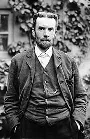
Let us pause explanations of Heaviside's achievements and focus on his biography and historical circumstances that surrounded his science breakthrough. Oliver Heaviside was born on May 18, 1850 in Camden Town, London, England. He caught scarlet fever when he was a young child and this affected his hearing. This was to have a major effect on his life, making his childhood unhappy, with relations between himself and other children difficult. However, his school results were rather good, and in 1865 he was placed fifth from five hundred pupils. Academic subjects seemed to hold little attraction for Heaviside, however, and at age 16 he left school. Perhaps he was more disillusioned with school than with learning since he continued to study (Oliver was completely self-taught) after leaving school, in particular he learned Morse code, studied electricity, and studied further languages, in particular Danish and German. He was aiming at a career as a telegrapher; in this he was advised and helped by his uncle Charles Wheatstone (the piece of electrical apparatus known as the Wheatstone bridge is named after him).
In 1868, Heaviside went to Denmark and became a telegrapher. He progressed quickly in his profession and returned to England in 1871 to take up a post in Newcastle upon Tyne in the office of Great Northern Telegraph Company, which dealt with overseas traffic. Heaviside became increasingly deaf but he worked on his own research into electricity. While still working as chief operator in Newcastle he began to publish papers on electricity, the first in 1872, and then the second in 1873, which was of sufficient interest to James Clerk Maxwell (1831--1879) that he mentioned the results in the second edition of his Treatise on Electricity and Magnetism. Despite this hatred of rigor, Heaviside was able to greatly simplify Maxwell's twenty equations with twenty variables, replacing them by four equations with two vector variables (the electric field E and the magnetic field B). Today we call these 'Maxwell's equations forgetting that they are in fact 'Heaviside's equations.'
Heaviside went on to achieve further advances in knowledge, again receiving less than his just desserts. In a 1887 paper Heaviside gave, for the first time, the conditions necessary to transmit a signal without distortion. In Electromagnetic Theory (1893--1912), he postulated that an electric charge would increase in mass as its velocity increases, an anticipation of an aspect of Einstein’s special theory of relativity. Heaviside was elected a Fellow of the Royal Society in 1891, perhaps the greatest honor he ever received. In 1902 Heaviside predicted that there was a conducting layer in the atmosphere which allowed radio waves to follow the Earth's curvature. This layer in the atmosphere, the Heaviside layer, is named after him. Its existence was proved in 1923 when radio pulses were transmitted vertically upward and the returning pulses from the reflecting layer were received.
⁎ ✱ ✲ ✳ ✺ ✻ ✼ ✽ ❋ ■On the eve of the twentieth century, new emerging physical ideas required new mathematical tools to formalize these theories. It is not an accident that many new mathematical notations and definitions were introduced by physicists, but not mathematicians. We cannot neglect to mention the famous Dirac's delta-function as well as the Einstein summation abbreviation. The latest example gave us the Internet, including the HTML protocol. Therefore, Heaviside's invention of operational calculus has naturally evolved to quantum mechanics and then as a byproduct, a useful technique for solving initial value problems for differential equations.
The Laplace transform is an integral transformation because it maps a function of a real variable t ∈ ℝ+ (as a rule, time) to a function of a complex variable λ (complex frequency):
To this day, the Inverse Laplace Transform is the most difficult process to understand when solving differential equations with the operational technique. In this tutorial, we will not use the formal definition of the inverse Laplace transform; instead, we apply the residue method based on the novel approach proposed by Vladimir Dobrushkin.
The revolutionary idea of Heaviside's operational calculus consists in establishing the spectral decomposition of the (unbounded) derivative operator \( \texttt{D} = {\text d}/{\text d} t \) acting in the space of functions on the half line [0, ∞). This means that the operator was replaced by simple multiplication. We will meet this approach in the second part of this tutorial when spectral decomposition will be applied to square matrices and second order differential operators.
Due to his research, Heaviside dealt with multi-degree differential equations for electrical systems in the 1880s. To solve corresponding initial value problems, Heaviside substituted the derivative operator by a letter p (we use the contemporary notation \( \texttt{D} \) instead), which yields algebraic equation. He then quickly solved the algebraic equation and proceeded with a solution to the original differential equation. These kinds of equations (usually with 10 or more derivatives of a dependent variable) would usually take days or weeks for most people to solve. Heaviside was able to solve these kinds of equations within hours. Between 1880--1887, he invented operational calculus -- a new method for solving the differential equations.
Unfortunately, Oliver Heaviside failed to explain how he had derived the solutions to the initial value problems, and as often happens the work of geniuses is not often understood. It took many years for academia to accept his results because of a lack of a rigorous proof for his methods. He replied to this criticism with the famous statement "Mathematics is an experimental science, and definitions do not come first, but later on," claiming that "I do not refuse my dinner simply because I do not understand the process of digestion." As a result, mathematicians did not accept his technique and tried to explain what is going on behind his manipulations. After many years of work, it became clear that Heaviside used the integral transformation.
Concept Overview
Note that this relation is valid only in a vector subspace of functions that vanish at the origin. Essentially, we will be doing almost the same thing that Heaviside had done-- we will take a linear differential equation, subject to the initial conditions
- Dobrushkin, V., Applied Differential Equations: the Primary Course, CRC Press,
- Hadamard, Jaques, Sur les problèmes aux dérivées partielles et leur signification physique. Princeton University Bulletin, 1902, pp. 49--52.
- Halmos, P.R., What does the spectral theorem say?, The American Mathematical Monthly, 1963, Vol. 70, No. 3, pp. 241--247.
- Iqbal, M., Classroom Note: Fourier method for Laplace transform inversion, Journal of Applied Mathematics and Decision Sience, 2001, Vol. 5, No. 3, pp. 193--200.
- O'Brien, K., Mathematics Magazine, 2018,