Return to computing page for the second course APMA0340
Return to computing page for the fourth course APMA0360
Return to Mathematica tutorial for the first course APMA0330
Return to Mathematica tutorial for the second course APMA0340
Return to Mathematica tutorial for the fourth course APMA0360
Return to the main page for the course APMA0330
Return to the main page for the course APMA0340
Return to the main page for the course APMA0360
Return to Part I of the course APMA0330
Glossary
Discontinuous Functions
There are two types of discontinuous functions. There are piecewise functions and functions that are discontinuous at a point. A piecewise function is a function defined by different functions for each part of the domain of the entire function (sometimes referred to as "the support," indicating the x axis in 2D). If the functions' individual domains do not use the entirety of the support, plotting them reveals they are separated by empty space..
A discontinuous function is a function that has a discontinuity at one or more values, often because of zero in the denominator. For example, if the denominator is (x−1), the function will have a discontinuity at x=1. Discontinuous functions are to be distinguished from "smooth" functions, the former exhibiting a hard corner at a particular point. Such function are not "differentiable everywhere" because the limit techniques which underlie derivative methodology do not work on hard corners.
Using Mathematica, it is easy to plot a piecewise discontinuous function.
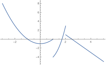
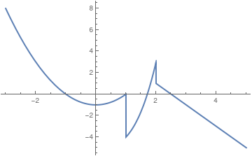
An example of a Piecewise function is given below. There are three different functions that have been generated in a single graph. Here are two options: either exclude discontinuities (which is a default option) or connect them (with option Exclusions)
Plot[Piecewise[{{x^2 - 1, x < 1}, {x^3 - 5, 1 < x < 2}, {5 - 2 x, x > 2}}], {x, -3, 5}, Exclusions -> {False}, PlotStyle -> Thick]
 |
 |
This code is very similar to the Plot command. The only difference is that you add the Piecewise Command and after
this command you enter the different components of the piecewise equation and the range for each of these components.
This code creates a graph that shows all three of the different piecewise components over the range of -3 to 5. Piecewise graphing does not create vertical lines at the boundary lines of each of the piecewise components.
You may want to put your plots into a frame,
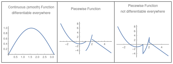
pltPW1 = Plot[Piecewise[{{x^2 - 1, x < 1}, {x^3 - 5, 1 < x < 2}, {5 - 2 x, x > 2}}], {x, -3, 5}, PlotLabel -> "Piecewise Function", PlotStyle -> Thick];
pltPW2 = Plot[ Piecewise[{{x^2 - 1, x < 1}, {x^3 - 5, 1 < x < 2}, {5 - 2 x, x > 2}}], {x, -3, 5}, PlotLabel -> "Piecewise Function\nnot differentiable everywhere", Exclusions -> {False}, PlotStyle -> Thick];
GraphicsRow[{pltSin, pltPW1, pltPW2}, AspectRatio -> Full, Frame -> All]
 |
Discontinuous functions can be plotted in Mathematica using the following command.
Plot[1/(x - 1), {x, 0, 2}, PlotStyle->{Thick,Blue}]
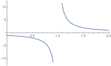
The latest version of Mathematica does not generate the vertical line of discontinuity (at x = 1 in our case). It can be added with Epilog
|
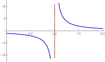
We add the vertical line with epilog:
line1 = Line[{{1, -11}, {1, 11}}];
lineStyle = {Thick, Red, Dashed}; Plot[1/(x - 1), {x, 0, 2}, PlotStyle -> {Thick, Blue}, Epilog -> {Directive[lineStyle], line1}] Another option:
line1 = Line[{{1, -11}, {1, 11}}];
lineStyle = {Thick, Red, Dashed}; Plot[1/(x - 1), {x, 0, 2}, PlotStyle -> {Thick, Blue}, Epilog -> {Directive[lineStyle], line1}] |
|
| Discontinuous function. | Mathematica code |
Another option is to use GridLines, which is an option for two-dimensional graphics functions that specifies grid lines:
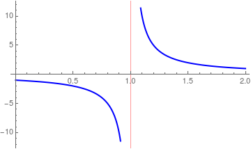
You can also relocate the origin:
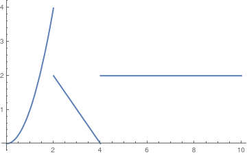
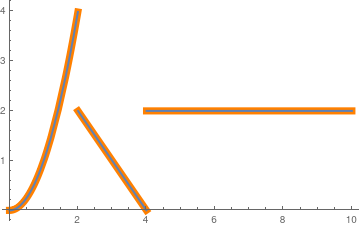
Let’s plot a piecewise function: \( f(t) = \begin{cases} t^2 , & \ 0 < t < 2 , \\ 4 - t, & \ 2 < t < 4, \\ 2, & t > 4. \end{cases} \)
The function is undefined at the points of discontinuity x = 1 and x = 4.
f[#] & /@ {2, 1.5, 3.7, 4.2}
pltF1 = Plot[f1[t], {t, 0, 10}, PlotRange -> Full, PlotStyle -> Thick]
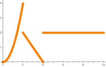
The same function with the value of 1 at t = 2:
 |
f2[t_] :=
Piecewise[{{Piecewise[{{t^2, 0 < t < 2}, {1, t == 2}}],
0 < t <= 2}, {Piecewise[{{4 - t, 2 < t < 4}, {2, t > 4}}], t > 2}}];
pltF2 = Plot[f2[t], {t, 0, 10}, PlotStyle -> {Thickness[.02], Orange}, PlotRange -> Full] |
|
| Graph of discontinuous function. | Mathematica code. |
These two plots are intended to be identical:
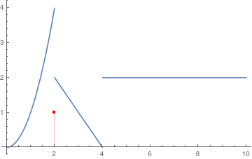 |
To show the discrete value at t = 2, we have two options:
pts := ListPlot[{{2, 1}}]
a := Plot[f2[t], {t, 0, 10}, PlotRange -> Full] Show[a, pts]
dp := DiscretePlot[1, {k, 2, 2}, PlotStyle -> Red]
Show[a, dp] |
|
| Graph of discontinuous function. | Mathematica code. |
Notice below the additional vertical line. This shows a discontinuous function on a sub-interval.
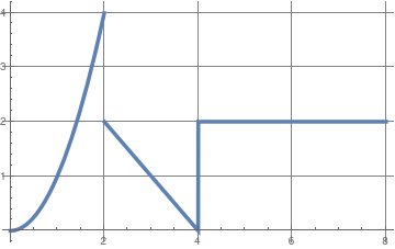 |
f3[t_] = Piecewise[{{t^2, 0 < t < 2}, {1, t == 2}, {4 - t,
2 < t < 4}, {2, t > 4}}];
Plot[f3[t], {t, 0, 8}, PlotRange -> All, GridLines -> Automatic, GridLinesStyle -> Directive, PlotStyle -> Thickness[0.01]] |
|
| Discontinuous function on the grid. | Mathematica code. |
We can also include the value of the function at one point (x = 2 in our case) into definition of the piecewise function.
f3[2]
We can find limits of this function at the point of discontinuity.
f[2]
Limit[f[x], x -> 2, Direction -> 1]
Limit[f[x], x -> 2, Direction -> -1]
Limit[f3[x], x -> 2, Direction -> 1]
We can redefine a function at one (or discrete number) point. Suppose we have the function \( \displaystyle f(x) = \frac{\left( x-1 \right) (x+3)}{x-1} . \) Mathematica is very smart and knows how to cancel out common terms:
Vertical and horizontal lines
To clear all definitions of quantities you've introduced in a Mathematica session so far, type: ClearAll["Global'*"].
The following command clears all the definitions made during the current Wolfram System session:
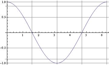
When you are graphing discontinuous functions, often times, it can be useful to generate a vertical or horizontal asymptote. To do this, you can use the following commands:
Plot[c,{x,c1,c2}] for horizontal asymptotes. In this command, c is the value of the horizontal asymptote and c1 and c2 are the range of the graph.
The following command clears all the definitions made during the current Wolfram System session:
Since a vertical line is not a graph of any function, so Plot won't help. However, Mathematica easily handles this challenge, while plotting a horizontal line is straight forward. We present several options to plot vertical lines
- The easiest way is to use Line command withing Graphics environment.
-
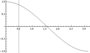
Another simple option is to utilize Rotate; just plot a horizontal line and then rotate it by π/2:
True, but you rotate the entire image, including the axes, effecting swapping the x for the y which changes the nature of the variables (independent or dependent).
 Rotate[Plot[y[x] = 0, {x, -1, 1}, PlotRange -> {-1, 1}, PlotStyle -> {Thickness[0.01], Red}], Pi/2]
 -
The command Line is suitable to plot a straight line in any direction, including vertical line.
The option InfiniteLine does not require you to know the plot range. - Epilog is very convenient to implement. While adding lines as Epilog (or Prolog) objects works most cases, the method can easily fail when automated, for example by automatically finding the minimum and maximum of the dataset.
-
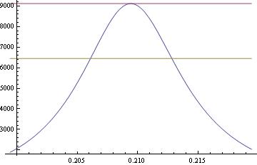
GridLines option works in all cases.
Plot[{f[x]}, {x, π/15 - 1/20, π/15 + 1/20}, GridLines -> {{π/15 + 1/50, π/15 - 1/50}, {f[π/15], f[π/15]/Sqrt[2]}}, PlotRange -> All]
-
Another possibility is to use Ticks:
Plot[{Sin[x], Cos[\[Pi]/3], Sin[\[Pi]/3]/Sqrt[2]}, {x, \[Pi]/3 - .06, \[Pi]/3 + .06}, Ticks -> {{{\[Pi]/3 + 1/20, \[Pi]/3 + 1/20, {0.595, 0}, Directive[Red, Dashed]}, {\[Pi]/3 - 1/20, \[Pi]/3 - 1/20, {0.595, 0}, Directive[Blue, Dashed]}}, All}, PlotRange -> {{0.12, 3}, All}]It is usually used with >TicksStyle.
-
Exclusions is a very helpful option when plotting a discontinuous function.
Plot[Tan[x], {x, 0, 6}, Exclusions -> {x == Pi/2, x == 3*Pi/2}, ExclusionsStyle -> Red]
-
ContourPlot is great to plot a vertical line.
ContourPlot[x == 0, {x, -1, 1}, {y, -1, 1}, Contours -> {Thick}, ContourStyle -> Red]
-
ParametricPlot solves this problem easily:
ParametricPlot[{3, t}, {t, -5, 5}, PlotRange -> 5]
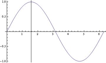
Mathematica can easily add the vertical line. The range of this function is 1 to 3. Then the command calls for Mathematica to create a straight vertical gridline at x=2. None is part of the command that tells Mathematica to just make it a straight dark, non dashed line.
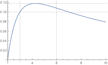
If you're actually using Plot (or ListPlot, etc.), the easiest solution is to use the GridLines option,
which lets you specify the x- and y-values where you want the lines drawn.
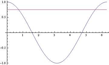
For the case of horizontal lines when using Plot the easiest trick is to just include additional constant functions
For vertical lines, there's the Epilog option for Plot and ListPlot:
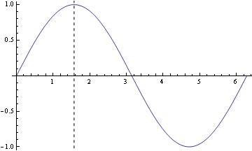
Another, perhaps even easier, option would be using GridLines:
f[x_] := (x^2 z)/((x^2 - y^2)^2 + 4 q^2 x^2) /. {y -> \[Pi]/15, z -> 1, q -> \[Pi]/600}
Plot[{f[x], f[\[Pi]/15],f[\[Pi]/15]/Sqrt[2]}, {x, \[Pi]/15 - .01, \[Pi]/15 + .01}]
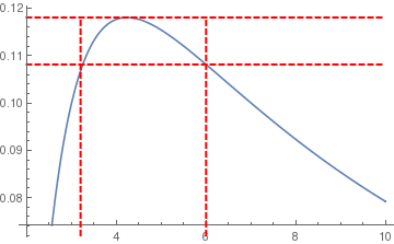
Another option to plot horizontal and vertical lines indicating the maximum value.
Quiet[maxy = FindMaximum[f[x], {x, 4}]]
lineStyle = {Thick, Red, Dashed};
line1 = Line[{{3.2, 0}, {3.2, maxy[[1]]}}];
line2 = Line[{{6, 0}, {6, maxy[[1]]}}];
Plot[{f[x], f[2 + Sqrt[5]], f[6]}, {x, 2, 10}, PlotStyle -> {Automatic, Directive[lineStyle], Directive[lineStyle]}, Epilog -> {Directive[lineStyle], line1, line2}]
Return to Mathematica page
Return to the main page (APMA0330)
Return to the Part 1 (Plotting)
Return to the Part 2 (First Order ODEs)
Return to the Part 3 (Numerical Methods)
Return to the Part 4 (Second and Higher Order ODEs)
Return to the Part 5 (Series and Recurrences)
Return to the Part 6 (Laplace Transform)
Return to the Part 7 (Boundary Value Problems)