Return to computing page for the first course APMA0330
Return to computing page for the second course APMA0340
Return to computing page for the fourth course APMA0360
Return to Mathematica tutorial for the first course APMA0330
Return to Mathematica tutorial for the second course APMA0340
Return to Mathematica tutorial for the fourth course APMA0360
Return to the main page for the course APMA0330
Return to the main page for the course APMA0340
Return to the main page for the course APMA0360
Return to Part V of the course APMA0330
Generally speaking, second-order differential equations with variable coefficients cannot be resolved in terms of the known functions. However, there is a fairly large class of differential equations whose solutions can be expressed either in terms of power series, or as simple combination of power series and elementary functions. It is this class of differential equations that we shall study in this chapter. For this, it is convenient to let the independent variable be x.
This section provides a stream of examples demonstrating applications of power
series method for solving initial value problems for second order differential
equations.
This section is devoting to series solutions of the second order differential equations. We start with linear differential equations. However, we first remind the important definition.
Definition: A
complex and single-valued function ƒ of a complex variable z is said to be holomorphic at a point 𝑎 if it is differentiable at every point within some open disk centered at 𝑎; this is equivalent that function ƒ can be expanded as a convergent power series with positive radius of convergence:
\[
f(x) = \sum_{n\ge 0} c_n \left( z - a \right)^n .
\]
Holomorphic functions are also sometimes referred to as regular functions.
A complex-valued function is said to be an analytic function if it is obtained from some holomorphic function by analytic continuation. An analytic function has all derivatives at any point from its domain (so it is a holomorphic in some disk), but it can be multi-valued consisting of at most countable number of branches (= holomorphic functions).
The word "holomorphic" was introduced by two of Cauchy's students, Briot (1817–1882) and Bouquet (1819–1895). Its name is derived from the Greek ὅλος (holos) meaning "entire", and μορφή (morphē) meaning "form" or "appearance".
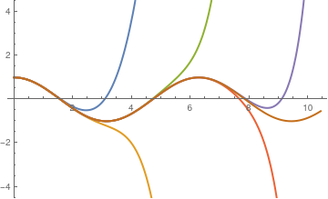
You studied in calculus some holomorphic functions---functions that are represented by connvergent power series. For example, a familiar cosine function has a Maclaurin series representation
Mathematica has a dedicated comamnd to determine a series approximation to solutions of linear equations. Since the cosine function is a solution to the initial value problem (IVP for short)
Some Maclaurin series approximations for cosine function
Linear Equations
There is an elegant Theorem, due to a Jewish-German mathematician Lazarus Fuchs (1833--1902) that guarantees existence of power series solutions to a linear differential equation of the second order which has the radius of convergence of the series solution at least as big as the minimum of the radii of convergence for its coefficients.
Fuchs's Theorem:
Consider the initial value problem for a linear differential equation of second order written in a normalized form
where prime stands for derivative with respect to independent variable x: \( y' = {\text d}y/{\text d}x . \)
Let r > 0. If both p(x) and q(x) have Taylor series, which converge on the interval
\( \left\vert x - x_0 \right\vert < 0, \)
then the differential equation has a unique power series solution y(x) that also converges on the same interval.
In particular, if both p(x) and q(x) are polynomials, then y(x) solves the differential equation for all x ∈ ℝ.
Definition: If in the linear differential equation \( y'' + p(x)\, y' + q(x) \,y =0 \) both coefficients, p(x) and q(x) are holomorphic at point x = x0, then this point x0 is called an ordinary point of the differential equation,
Suppose that the coefficients p(x) and q(x) can be developed into power series
Note that if p(x) and q(x) are polynomials of degree at most m, then the recurrence relation for determination of coefficients becomes a difference equation of order m.
Example 1:
Let us consider an initial value problem (IVP) for a homogeneous linear differential equation:
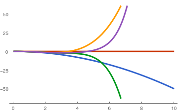
We set up our Taylor series as a symbolic expansion using derivatives of x evaluated at the origin. I use an order of 15 but that is something one would probably make as an argument to a function, if automating all this.
zz = Series[y[x], {x, 0, 15}];
Next apply the differential operator and add the initial conditions. Then find a solution that makes all powers of x vanish.
This is a good start. Power series solutions, though, are frequently used to obtain recursion equations for the coefficients (of any solution that might be analytic within a neighborhood of the point of expansion). It would be nice, then, to have a function that outputs these equations (given a differential operator as input), rather than just obtaining an approximate solution with a limited radius of accuracy. In order to analyze singular points, it would also be useful to consider slightly more general series of the Frobenius form
are holomorphic functions in the circle |x - 2| < 2. Therefore, we expect that our differential equation has a solution that can be represented by a convergent in the same circle series:
This is a general solution composed by two linearly independent solutions, where c0, c1 are arbitrary constants.
Use of the nearest singular point is of some worth since having a lower bound is stronger than not knowing anything about the radius of convergence. However, for particular types of differential equations, there is a method that has been proven to give an exact value.
■
Example 4:
Let us consider a second order differential equation
\[
y'' + x^2 y' - x^3 y = 0.
\tag{4.1}
\]
We are going to determine a lower bound on the radius of convergence for the series solution about x0 = 0 and x0 = 3.
The point x0 = 0 is an ordinary point since the coefficients of the given differential equation \( \displaystyle y'' + p(x)\, y' + q(x)\, y = 0 \) are holomorphic functions:
The radius of convergence of the series solution will be at least as large as the minimum of the radius of convergence of the
series for p(x) = (x² and q(x) = (x³ about x0 = 0.
Since p(x) and q(x) are already expanded in power series, and these series are not infinite, the radius of convergence for
them is ρ = ∞. Therefore, the series solution about x0 = 0 must have a radius of convergence that is at least as large as ρ = ∞, which of
course means it must be ρ = ∞.
A similar argument holds for x0 = 3.
■
Example 5:
Let us consider a second order differential equation
Let’s determine the radius of convergence of p and q without working out the Taylor series for them.
The complex poles of p and p all occur when x² −x + 3 = 0, which means x = 1 and x = −3.
These roots are at distance 1 and 3 from the origin.
Since the nearest complex pole is 1, we conclude that the radius of convergence of the series for p(x) and q(x) is ρ = 1. Therefore, the minimum radius of convergence for the series solution about x0 = 0 to the differential equation is ρ = 1.
The distance from x0 = 5 to the nearest complex pole is ρ = 4. The minimum radius of convergence for the series solution about x0 = 5 to the differential equation is ρ = 4.
■
Nonlinear Equations
Example 6:
The conservative form of the Burgers' equation can be reduce to the following form
\[
v\,v' = \nu\,v'' ,
\]
where ν is a positive constant.
Substituting the proposed series solution
Solving the algebraic system of 9 equations, for the 9 unknown variables
[a2, a3, ... ,a9]
as functions of two known initial values a0 =
v(0) and a1 = v'(0) and the
physical parameterν, we express coefficients explicitly:
We can rewrite the Duffing equation in the operator form:
\[
L\left[ y \right] \equiv \texttt{D}^2 y = N \left[ y \right] \equiv
\varepsilon \,y^3 - k\, y.
\]
Physically, the resilience of the oscillator is directly proportional to
N[y]. When k ≥ 0 and ε < 0, there is one
unique equilibrium point y = 0 where the nonlinear term vanishes.
However, when k ≤ 0 and ε > 0, there are two
equilibrium points: y = 0 and
\( y = \sqrt{|k/\varepsilon |} . \)
From the physical points of view, the sum of the kinetic and
potential energy of the oscillator keeps the same, therefore it is clear that
the oscillation motion is periodic, no matter k is positive or
negative. Thus, from physical points of view, it is easy to know that
y(t) is periodic, even if we do not directly solve the Duffing
equation.
■
Example 8:
Example: Move to chapter 4, ndsolve
Consider the second-order nonlinear
differential equation with the product of the derivative
and a sinusoidal nonlinearity of the solution
This equation arises from the general sine-Gordon equation
\[
u_{tt} - u_{xx} - \sin u =0 ,
\]
which is a model for the nonlinear meson fields with periodic properties for the unified description of mesons and their particle sources. A simple solution of the sine-Gordon equation may be found by representing u as a function of
\( \xi = \left( x - vt \right) /\sqrt{1-v^2} . \) In this case, the sine-Gordon equation is reduced to the pendulum like equation
\( {\text d}^2 u/{\text d} \xi^2 = \sin u . \) For a real physical velocity v < 1, there are implicit solutions given by
with total energy
\( \displaystyle E = \frac{2}{\pi} \,\frac{1}{\sqrt{1-v^2}} . \) These solutions may be interpreted as the fields associated with a particle of mass 2/π centered at ξ = ξ0 and moving with velocity v.
■
Exampl 10:
The system of partial differential equations, called KdV equations, can be
reduced by appropriate substitution to the following ordinary differential
equation
\[
v' = k\,v''' - v\,v' .
\]
■
In all problems, y' denotes the derivative of function y(x) with respect to independent variable x and \( \dot{y} = {\text d} y/{\text d}t \) denotes the derivative with respect to time variable.
Using ADM, solve the initial value problem: \( e^x \,y'' + x\,y = 0 , \quad y(0) =A, \quad y' (0) = B . \)
Using ADM, solve the initial value problem: \( e^x \,y'' + x\,y = 0 , \quad y(0) =A, \quad y' (0) = B . \)
Grigorieva, E., Methods of Solving Sequence and Series Problems, Birkhäuser; 1st ed. 2016.
Return to Mathematica page
Return to the main page (APMA0330)
Return to the Part 1 (Plotting)
Return to the Part 2 (First Order ODEs)
Return to the Part 3 (Numerical Methods)
Return to the Part 4 (Second and Higher Order ODEs)
Return to the Part 5 (Series and Recurrences)
Return to the Part 6 (Laplace Transform)
Return to the Part 7 (Boundary Value Problems)