Return to computing page for the second course APMA0340
Return to computing page for the fourth course APMA0340
Return to Mathematica tutorial for the first course APMA0330
Return to Mathematica tutorial for the second course APMA0340
Return to the main page for the course Return to Mathematica tutorial for the fourth course APMA0340
APMA0330
Return to the main page for the course APMA0340
Return to the main page for the course APMA0360
Return to Part V of the course APMA0330
Glossary
Preface
Figures with Arrows
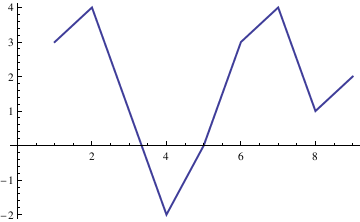
When one wants to plot a figure that is built from straight lines, it can be done as follows
|
ListLinePlot[{3, 4, 1, -2, 0, 3, 4, 1, 2}, PlotStyle->Thick]
|
|
| LinePlot in action. | Mathematica code |
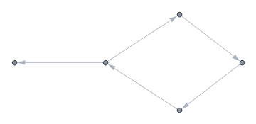
A directed graph can be plotted as well
|
Graph[{1 -> 3, 1 -> 2, 2 -> 4, 4 -> 5, 5 -> 1}]
|
|
| Directed graph. | Mathematica code |
|
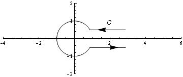
With[{q = Pi/6},
Graphics[{Circle[{0, 0}, 1, {q, 2 Pi - q}], Arrowheads[{{.05, .8}}], Arrow[{{Cos[q] + 2, Sin[q]}, {Cos[q], Sin[q]}}], Arrow[{{Cos[q], Sin[-q]}, {Cos[q] + 2, Sin[-q]}}], FontSize -> Medium, Text["\[ScriptCapitalC]", {2, Sin[q]}, {0, -2}]}, Axes -> True, PlotRange -> {{-4, 6}, {-2, 2}}]] |
|
| Traverse a cut. | Mathematica code |
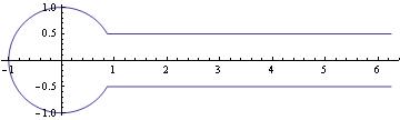
If you want to plot the actual contour without arrows, then try something like the following:
|
contour[t_, t0_: (5 Pi/6)] := Piecewise[{ {Exp[I (t + Pi)], -t0 < t < t0},
{t - t0 + Exp[I (t0 + Pi)], t >= t0}, {-t - t0 + Exp[-I (t0 + Pi)], t <= -t0}}] ParametricPlot[Through[{Re, Im}[contour[t]]], {t, -8, 8}, PlotPoints -> 30] |
|
| Traverse a cut. | Mathematica code |
Another option:
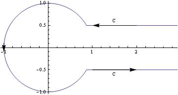
|
c = 0.5;
t0 = ArcSin[c]; PolarPlot[If[Abs[t] < t0, Abs[Sin[t0]/Sin[t]], 1], {t, -\[Pi], \[Pi]}, Epilog -> { Arrow[{{2, c}, {1, c}}], Arrow[{{1, -c}, {2, -c}}], Arrow[{{-1, .1}, {-1, -.1}}], Text["C", {1.5, c + .1}], Text["C", {1.5, -(c + .1)}] }] |
|
| Traverse a cut. | Mathematica code |
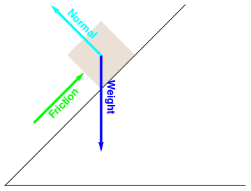
Now we show how to add arrows into the graph.
g2=Graphics[Line[{{0,0},{15,15}}]]
g3=Graphics[{Opacity[0.2],Brown,Rotate[Rectangle[{8,8},{12,12}], 45 Degree, {Left, Bottom}]}]
g4=Graphics[{Blue, Thickness[0.01], Arrow[{{8,10.8}, {8,2.8}}]}]
g5=Graphics[{Cyan, Thickness[0.01], Arrow[{{8,10.8}, {3.8,15}}]}]
g6=Graphics[{Green, Thickness[0.01], Arrow[{{2.4,5.2}, {6.6,9.4}}]}]
g7 = Graphics[ Text[StyleForm["Weight", FontSize -> 14, FontWeight -> "Bold", FontColor -> Blue], {9.4, 6.8}, {0.4, 1}, {0, -1}]]
g8=Graphics[ Text[StyleForm["Normal", FontSize -> 14, FontWeight -> "Bold", FontColor -> Cyan], {6, 13}, {0, -1}, {1, -1}]]
g9=Graphics[ Text[StyleForm["Friction", FontSize -> 14, FontWeight -> "Bold", FontColor -> Green], {4.5, 7.2}, {0, 1}, {1, 1}]]
Show[g1,g2,g3,g4,g5,g6,g7,g8,g9]
|
|
ContourPlot[x^2 + y^2 == 9, {x, -2, 2}, {y, -2, -3.1},
AspectRatio -> 0.5] /.
Line[x__] :> Sequence[Arrowheads[{-.04, .04}], Arrow[x]] |
|
| Curve with arrows. | Mathematica code |
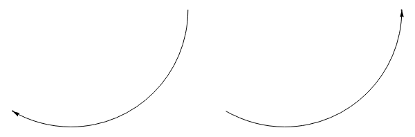
We can add arrows to multiple plots:
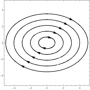
|
rules = {GraphicsComplex[x_, y_] :>
GraphicsComplex[SortBy[x, ArcTan[#[[1]], #[[2]]] + (\[Pi]/2) &], y /. Line[pts_] :> {Arrowheads[{{-0.05, 1/8}, {-0.05, 5/8}}], Arrow[pts]}]} Show @@ Table[ ContourPlot[x^2 + 2*y^2 == r^2, {x, -r, r}, {y, -r, r}, PlotPoints -> 100, ContourShading -> False, ContourStyle -> {Black, Thick}] /. rules, {r, 5, 1, -1}] |
|
| Family of curves with arrows. | Mathematica code |
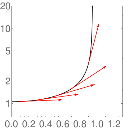
To add uniform arrows to the graph, we use Alexey Popkov's completePlotRange for computing the actual PlotRange of a plot.
Last@Last@
Reap[Rasterize[
Show[plot, Axes -> True, Frame -> False,
Ticks -> ((Sow[{##}]; Automatic) &),
DisplayFunction -> Identity, ImageSize -> 0],
ImageResolution -> 1]]
|
Block[{f, f0, df0, ar, plot}, f = (0.9 - x^2)^(-0.5);
f0 = Log[f] /. x -> x0; df0 = D[Log[f], x] /. x -> x0; plot = LogPlot[f, {x, 0, 1}, PlotRange -> {{0, 1.3}, {0.66, 20}}, Frame -> {{True, True}, {True, False}}, ImageSize -> 400, PlotStyle -> {Directive[Black, Thick], Automatic}, BaseStyle -> {FontSize -> 30}, RotateLabel -> False, AspectRatio -> 1]; ar = If[(AspectRatio /. Options[plot, AspectRatio]) === Automatic, 1, (AspectRatio /. Options[plot, AspectRatio])/ Ratios[Differences /@ completePlotRange@plot][[1, 1]]]; Show[plot, Graphics[{Red, Thick, Table[Arrow[{{x0, f0}, {x0, f0} + 0.5 {1, df0}/Norm[{1, df0*ar}]}], {x0, 0.1, 0.9, 0.2}]}]]] |
|
| Demonstration of Popkov's block. | Mathematica code |
|
|
Now we show how to plot figure when arrows are attached to curves/circles.
Show[ParametricPlot[#[[1]]*{Cos[θ], Sin[θ]}, {θ, #[[2]], #[[3]]},
Axes -> False, PlotStyle -> #[[4]]] /. Line[x_] :> Sequence[Arrowheads[{-0.05, 0.05}], Arrow[x]] & /@ {{1, 0 Degree, 90 Degree, Red}, {1.25, 0 Degree, 270 Degree, Blue}, {1.5, 0 Degree, 180 Degree, Green}}, PlotRange -> All] |
|
| Circles with arrows. | Mathematica code |
|
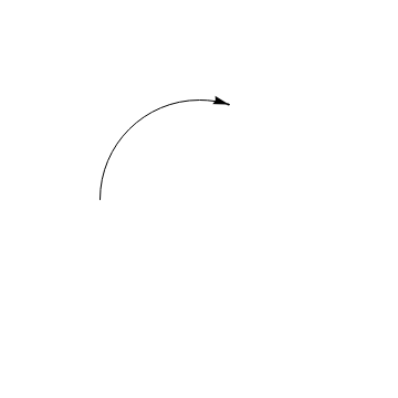
Here is another block of codes with Manipulation option that allows you to change the size of arc.
start = \[Pi];
Manipulate[ Graphics[{Arrow[{{Cos[\[Theta] + If[\[Theta] < start, .01, -.01]], Sin[\[Theta] + If[\[Theta] < start, .01, -.01]]}, {Cos[\[Theta]], Sin[\[Theta]]}}], Circle[{0, 0}, 1, {start, \[Theta]}]}, PlotRange -> 2], {{\[Theta], .7 start}, 0, 2 start}] |
|
| An arc with an arrow. | Mathematica code |
|
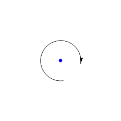
When you need to see the center of the circle, use the folloiwng code:
Manipulate[
Graphics[{arcArrow[center, radius, {start, end}], PointSize[Large], Blue, If[showCenter, Point[center]]}, PlotRange -> p, ImageSize -> 250], {{start, \[Pi]/2}, -2 \[Pi], 2 \[Pi], ImageSize -> Small}, {{end, 0}, -2 \[Pi], 2 \[Pi], ImageSize -> Small}, {{radius, 1}, 1/2, 4, ImageSize -> Small}, {{center, {0, 0}}, {-p, -p}, {p, p}, Slider2D}, {showCenter, {True, False}}, Initialization :> {p = 3; arcArrow[a_, r_, {start_, end_}] := {Circle[a, r, {start, end}], Arrowheads[Medium], Arrow[{a + r {Cos[end + If[end < start, .01, -.01]], Sin[end + If[end < start, .01, -.01]]}, a + r {Cos[end], Sin[end]}}]}}] |
|
| An arc with an arrow and the center. | Mathematica code |
Using Circle, define the function f (or whatever you want)
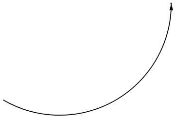
|
Concave up:
Graphics@{Thickness[0.005], f[Circle[{0, 0}, 1, {4 Pi/3, 2 Pi}]]}
|
|
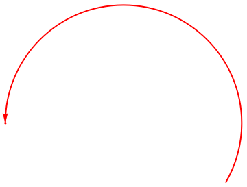
Concave down:
Graphics@{Red, Thick, f[Circle[{0, 0}, 1, {- Pi/6, Pi}]]}
|
You can use Circle directly with anderfining procedure:
arcsWArrows[args1 : {{_, {_, _}} ..},
dir_List: {Directive[GrayLevel[.3],
Arrowheads[{{-0.05, 0}, {0.05, 1}}]]}] :=
ParametricPlot[
Evaluate[#[[1]]*{Cos[Rescale[u, {0, 2 Pi}, Abs@#[[2]]]],
Sin[Rescale[u, {0, 2 Pi}, Abs@#[[2]]]]} & /@ args1], {u, 0,
2 Pi}, PlotStyle -> dir, Axes -> False, PlotRangePadding -> .2,
ImageSize -> 200] /. Line[x_, ___] :> Arrow[x]
2}}, {1.25, {0, \[Pi]}}, {1.5, {0, (3 \[Pi])/2}}, {2, {\[Pi]/
4, (4 \[Pi])/2}}};
directives = {Directive[Red, Thick,
Arrowheads[{{-0.05, 0}, {0.05, 1}}]],
Directive[Blue, Dashed, Arrowheads[{{-0.05, 0}, {0.05, 1}}]],
Directive[Green, Arrowheads[{{-0.05, 0}, {0.05, 1}}]],
Directive[Orange, Thickness[.02], Arrowheads[{{-0.07, 0}, {0.07, 1}}]]};
Row[{arcsWArrows[rdsAndAngls],
arcsWArrows[rdsAndAngls, {directives[[1]]}],
arcsWArrows[rdsAndAngls, directives],
arcsWArrows[rdsAndAngls, directives[[-1 ;; 2 ;; -1]]]}]
|
|
|
|
|
|
Show[
Graphics[{Lighter@Pink, AbsoluteThickness@10, Circle[o, r, {α Degree, β Degree}]}],
Graphics[{Arrow[pts, 0]}],
PlotRange -> {{-1.3, 1.3}, {-1.3, 1.3}}, AspectRatio -> 1,
Axes -> True, ImageSize -> 250 ],
{{d, 20, "res."}, 1, 100, Appearance -> "Labeled"},
{{α, 0, "α"}, 0, 360, Appearance -> "Labeled"},
{{β, 250, "β"}, 0, 360, Appearance -> "Labeled"},
{{r, 1, "r"}, 0.01, 2, Appearance -> "Labeled"},
{{o, {0, 0}, "origo"}, {-1, -1}, {1, 1}},
ControlPlacement -> Left ]
We plot a function that has the graph with ended arrows.
|
|
f[x_] := Sin[12 x^2]; xmin = -1; xmax = 1; small = .01;
Plot[f[x], {x, xmin, xmax}, PlotLabel -> y == f[x], AxesLabel -> {x, y}, Epilog -> {Blue, Arrow[{{xmin, f[xmin]}, {xmin - small, f[xmin - small]}}], Arrow[{{xmax, f[xmax]}, {xmax + small, f[xmax + small]}}]}] |
|
| Graph ends with arrows. | Mathematica code |
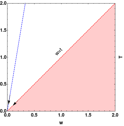
Finally, we demontrate some examples of plotting with text and arrows.
|
P1 = Plot[x, {x, 0, 2}, PlotStyle -> {Dashed, Red}, Filling -> Bottom];
P2 = Plot[6 x, {x, 0, 2}, PlotStyle -> {Dashed, Blue}];
Show[P1, P2, AspectRatio -> Automatic, Frame -> True,
PlotRangePadding -> None, AxesOrigin -> {0, 0}, Axes -> None,
FrameStyle -> Directive[Black], LabelStyle -> {18, Bold},
FrameLabel -> {{None, "T"}, {"w", None}}, ImageSize -> 500,
Epilog -> {
Arrow[{{.2, .2}, {.1, .1}}],
Arrow[{.05 {1, 6}, {1, 6} .02}],
Rotate[Text[Style["w=t", FontSize -> 20], {.95, 1.1}], Pi/4]}]
|
Text with arrows using Plot
|
Mathematica code |
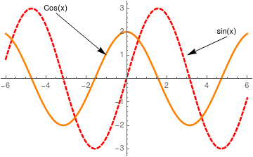
Another example:
|
Plot[{3 Sin[x], 2*Cos[x]}, {x, -6, 6},
PlotStyle -> {{Thickness[0.007], Dashed, Red}, {Thickness[0.007],
Orange}},
Epilog -> {{Arrow[{{5, 1.8}, {3, 1}}], Text["sin(x)", {5, 2}],
Arrow[{{-3.5, 2.8}, {-1, 1}}], Text["Cos(x)", {-3.5, 3}]}}]
|
Text with arrows using Plot
|
Mathematica code |
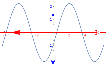
|
arrowhead1 = Polygon[{{-1, 0.5`}, {0, 0}, {-1, -0.5`}}];
arrowhead2 = Polygon[{{-1.5833333333333333`, 0.4166666666666667`}, {-1.5410500000000003`, 0.369283333333333`}, {-1.448333333333333`, 0.255583333333333`}, {-1.3991000000000005`, 0.18721666666666673`}, {-1.3564666666666663`, 0.11826666666666673`}, {-1.3268499999999999`, 0.05408333333333341`}, {-1.3166666666666667`, 0.`}, {-1.3268499999999999`, -0.048950000000000195`}, \ {-1.3564666666666663`, -0.11228333333333372`}, {-1.3991000000000005`, \ -0.18353333333333333`}, {-1.448333333333333`, -0.2562833333333335`}, \ {-1.5410500000000003`, -0.38048333333333345`}, {-1.5833333333333333`, \ -0.43333333333333335`}, {0.`, 0.`}, {-1.5833333333333333`, 0.4166666666666667`}, {-1.5833333333333333`, 0.4166666666666667`}}]; arrowhead3 = Polygon[{{-1, 0.5`}, {0, 0}, {-1, -0.5`}, {-0.6`, 0}, {-1, 0.5`}}]; arrowhead4 = {{FaceForm[GrayLevel[1]], Polygon[{{-0.6`, 0}, {-1.`, 0.5`}, {0.`, 0}, {-1.`, -0.5`}, {-0.6`, 0}}], Line[{{-0.6`, 0}, {-1.`, 0.5`}, {0.`, 0}, {-1.`, -0.5`}, {-0.6`, 0}}]}}; arrowhead5 = Polygon[{{-0.6582278481012658`, -0.43037974683544306`}, {0.`, 0.`}, {0.`, 0.`}, {0.`, 0.`}, {0.`, 0.`}, {0.`, 0.`}, {-0.6455696202531646`, 0.43037974683544306`}, {-0.4810126582278481`, 0.`}, {-0.6582278481012658`, -0.43037974683544306`}, \ {-0.6582278481012658`, -0.43037974683544306`}}]; Plot[2*Sin[x] - Cos[x], {x, -2 \[Pi], 2 \[Pi]}, AxesStyle -> {Directive[{Red, Arrowheads[{{-0.06, 0.1(*Xleft*), {Graphics[{arrowhead}] /. arrowhead -> arrowhead2, 0.98`}}, {0.05, 0.95(*Xright*), {Graphics[{arrowhead}], 0.98`}}}] /. arrowhead -> arrowhead4}], Directive[{Blue, Arrowheads[{{-0.05, 0(*Ydown*), {Graphics[{arrowhead}] /. arrowhead -> arrowhead3, 0.98`}}, {0.03, .8(*Yup*), {Graphics[{arrowhead}] /. arrowhead -> arrowhead1, 0.98`}}}]}]}] |
|
| Demonstration of arrows. | Mathematica code |
|
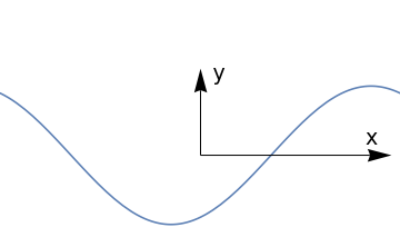
axes[x_, y_, f_, a_] :=
Graphics[Join[{Arrowheads[a]}, Arrow[{{0, 0}, #}] & /@ {{x, 0}, {0, y}}, {Text[ Style["x", FontSize -> Scaled[f]], {0.9*x, 0.2*y}], Text[Style["y", FontSize -> Scaled[f]], {0.1 x, 0.95*y}]}]] Show[Plot[1/2*Sin[x] - Cos[x], {x, -\[Pi], \[Pi]}, Axes -> None, PlotRange -> {{-Pi, Pi}, {-1.5, 2.5}}], axes[3, 1.4, 0.05, 0.06]] |
|
| Figure with coordinate arrows. | Mathematica code |
Plot with custom arrowheads:
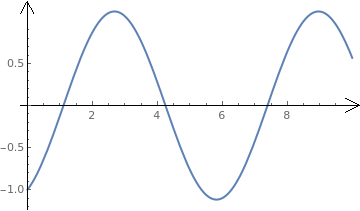
|
h = Graphics[Line[{{-1, 1/2}, {0, 0}, {-1, -1/2}}]];
Plot[1/2*Sin[x] - Cos[x], {x, 0, 10}, PlotStyle -> Thick, AxesStyle -> Arrowheads[{{Automatic, Automatic, h}}]] |
|
| Plot with custom arrowsheads. | Mathematica code |
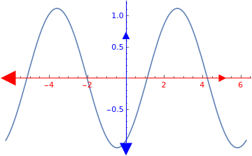
|
Plot[1/2*Sin[x] - Cos[x], {x, -2 \[Pi], 2 \[Pi]},
AxesStyle -> {Directive[{Red, Arrowheads[{{-0.06, 0(*Xleft*), {Graphics[{Polygon[{{-1, 0.5`}, {0, 0}, {-1, -0.5`}}]}], 0.98`}}, {0.03, .9(*Xright*), {Graphics[{Polygon[{{-1, 0.5`}, {0, 0}, {-1, -0.5`}}]}], 0.98`}}}]}], Directive[{Blue, Arrowheads[{{-0.05, 0(*Ydown*), {Graphics[{Polygon[{{-1, 0.5`}, {0, 0}, {-1, -0.5`}}]}], 0.98`}}, {0.03, .8(*Yup*), {Graphics[{Polygon[{{-1, 0.5`}, {0, 0}, {-1, -0.5`}}]}], 0.98`}}}]}]}] |
|
| Plot with triangle arrowsheads. | Mathematica code |
Return to Mathematica page
Return to the main page (APMA0330)
Return to the Part 1 (Plotting)
Return to the Part 2 (First Order ODEs)
Return to the Part 3 (Numerical Methods)
Return to the Part 4 (Second and Higher Order ODEs)
Return to the Part 5 (Series and Recurrences)
Return to the Part 6 (Laplace Transform)
Return to the Part 7 (Boundary Value Problems)