Return to computing page for the first course APMA0330
Return to computing page for the second course APMA0340
Return to computing page for the fourth course APMA0360
Return to Mathematica tutorial for the first course APMA0330
Return to Mathematica tutorial for the second course APMA0340
Return to Mathematica tutorial for the fourth course APMA0360
Return to the main page for the course APMA0330
Return to the main page for the course APMA0340
Return to the main page for the course APMA0360
Theorem 1::
Consider the first order differential equation
\( {\text d}y/{\text d}x = f(y) , \) where f
is continuous in a neighborhood of y0. Assume that the
solutions through y0 are not unique, that is, assume that
there are two solutions φ1 and φ2 such that
φ1(0) = φ2(0) = y0 amd that
φ1 and φ2 differ in every
neighborhood of 0. Than f(y0) = 0.
▣
Theorem 2:: Let f(y) be a continuous function on the closed interval [𝑎, b] that has one null \( y^{\ast} \in (a,b) , \) namely, \( f(y^{\ast} ) =0 \) and \( f(y) \ne 0 \) for all other points \( y \in (a,b) . \) If the integral
\[
\int_y^{y^{\ast}} \frac{{\text d}y}{f(y)}
\]
diverges, then the initial value problem for the autonomous differential
equation
\[
y' = f(y) , \qquad y(x_0 ) = y^{\ast}
\]
has the unique solution \( y (x) \equiv y^{\ast} . \) If the integral converges, then the initial value problem has multiple solutions.
▣
Theorem 3::
Suppose that
f(x,y) is uniformly Lipschitz continuous in y (meaning the Lipschitz constant L in the inequality \( |f(x,y_1 ) - f(x, y_2 )| \le L\,|y_1 - y_2 | \) can be taken independent of x) and continuous in x. Then, for some positive value δ there exists a unique solution \( y = \phi (x) \) to the initial value problem
\[
y' = f(x,y) , \qquad y(x_0 ) = y_0
\]
on the interval \( \left[ x_0 -\delta , x_0 + \delta \right] . \)
▣
Proof:
Suppose the the initial value problem
\( y' = f(x,y), \quad y(x_0 ) = y_0 , \)
with Lipschitz slope function f(x,y) has two solutions
y1 and y2. Let
\[
u(x) = \int_{x_0}^x \left\vert y_1 (s) - y_2 (s) \right\vert {\text d} s \ge 0
\quad \mbox{for} \quad x\ge x_0 .
\]
Since these functions are solutions of the same differential equation, they
also satisfy the equivalent integral equation
Therefore \( u(x) \le 0 , \) which leads to
conclusion that \( u(x) \equiv 0 \) for all
x ≥ x0.
A similar argument shows also that
\( u(x) \equiv 0 \) for all
x ≤ x0.
▣
Theorem 4::
Let R be the region defined by the inequalities
\( 0 \le x- x_0 < a, \ |s_k - y_k | < b_k , \quad k=0,1,2,\ldots , n-1 , \) where yk ≥ 0 for k
> 0. Suppose the function
\( f(x, s_0 , s_1 , \ldots , s_{n-1} ) \) in the
initial value problem
then the above initial value problem has at most one solution in R.
▣
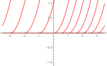
Example 1:
Consider the initial value problem
\[
y' = 2\,\sqrt{y}, \quad y(0)=0 ,
\]
where the slope function \( f(y) = 2\,\sqrt{y} \) is continuous on infinite interval \( [0, \infty ) \) but not Lipschitz. So according to Peano's theorem, this initial value problem has a solution. Indeed, we can apply Picard's iteration procedure to obtain a solution \( y(x) \equiv 0 . \) On the other hand, since the given differential equation is autonomous, we can separate variables and integrate:
where C is an arbitrary constant. Since we consider only positive branch of the square root function, the above formula is valid only when \( x \ge C . \) Therefore, we get a family of solutions (which is also called the general solution) depending on a parameter C:
\[
y = \begin{cases} \left( x-C \right)^2 , & \qquad x \ge C , \\
0 , & \quad \mbox{for } x <C . \end{cases}
\]
In this sequence of command, I am first entering the family of solutions to the differential equation. Since using C is prohibited in Mathematica, we use CC instead. Then we use two subroutines, one for plotting solutions, and another one for looping with respect to constant C, Finally, we display all graphs.
We can also check that the given initial value problem has multiple solutions by evaluating integral
It has again a trivial solution y(x) = 0. Let
\( u = y^{(n-1)} , \) then u(x) is
defined from the equation
\[
x = \int_0^u t^{-2/3} e^{-t}\,{\text d}t .
\]
As \( u \to \infty , \quad x\to r_0 = \int_0^{\infty}
t^{-2/3} e^{-t}\,{\text d}t . \) Then another solution is given by
\[
y(x) = \int_0^x \frac{\left( x - t \right)^{n-2}}{(n-2)!} \, u(t)\,{\text d}t ,
\]
defined on 0 ≤ x < r0 < ∞.
The function y(x) can be multiplied by arbitrary continuous, nonnegative, nondecreasing function of x to give other example.
■
It should be noted that the Lipschitz condition is a sufficient one but not a necessary condition for uniqueness. As an example where there exists unique solution in spite of the Lipschitz condition not being satistied is given by the initial value problem
\[
y' + 1 + (4/3) \,x^{1/3} , \qquad y(0) = 0.
\]
It is obvious that the slope function violates the Lipschitz condition in a domain which includes the origin. However the above initial value problem has a unique solution.
Example 4:
Following Dhar, we consider one dimensional motion modeled by Newton's equation
where \( \ddot{x} = {\text d}^2 x/{\text d}xt^2 \)
is acceleration of a unit point mass. It is always assun=mewd that functions
Π(x) and f(x) = - dΠ(x)/dx are
continuous functions of x.
We consider the case when the potential function Π(x) has a single
singularity at the origin in sense that \( V'' (x) \)
or one of the higher derivatives does not exist. So we consider the
initial value problem
where \( E = v_0^2 /2 \) is the total energy of the
system and is a constant because Π(0) = 0. The sign of the square roots
dependes on the sign of the initial velocity v0.
The first order differential equation \( \dot{x} = g(x)
\) is equivalent to Newton's equation \( \ddot{x} =
f(x) \) only if the velocity is not zero because we multiplied by
\( \dot{x} . \) Therefore, we need to consider two
cases depending whether the initial velocity is zero or not.
v0 ≠ 0. Then E0 ≠ 0 and the
reciprocal 1/g(x) is finite and continuous in an interval containing the origin. Therefore, the first order differential equation
\( \dot{x} = g(x) \) can be integrated to give the unique solution \( t = \int_0^x {\text d}\xi/g(\xi ) . \) So the second order equation of motion \( \ddot{x} =
f(x) \) will have a unique solution irrespective of the type of singularity that Π(x) may have.
v0 = 0, then E0 = E = 0 and the first order equation becomes
are real and finite. When these integrals exist, the second order differential equation of motion will have additional solution provided that f(0) = 0.
Now we formulate the necessary and sufficient conditions for the existence of unique solutions to the IVP for Newton's equation of motion:
■
Dhar, A., Nonuniqueness in the solutions of Newton's equation of motion, American Journal of Physics, 1993, Vol. 61, No. 1, pp. 58--61; doi: 10.1119/1.17411
Hales, A.W. and Sells, G.R., Multiple solutions of a differential equation,
The American Mathematical Monthly, 1966, Vol. 73, No. 6, pp.672--673.
Wend, D.V.V., Uniqueness of solutions of ordinary differential equations,
The American Mathematical Monthly, 1967, Vol. 74, No. 8, pp. 948--950.
Return to Mathematica page
Return to the main page (APMA0330)
Return to the Part 1 (Plotting)
Return to the Part 2 (First Order ODEs)
Return to the Part 3 (Numerical Methods)
Return to the Part 4 (Second and Higher Order ODEs)
Return to the Part 5 (Series and Recurrences)
Return to the Part 6 (Laplace Transform)
Return to the Part 7 (Boundary Value Problems)