Return to computing page for the second course APMA0340
Return to Mathematica tutorial for the first course APMA0330
Return to Mathematica tutorial for the second course APMA0340
Return to the main page for the course APMA0330
Return to the main page for the course APMA0340
Return to Part V of the course APMA0330
Glossary
Famous Curves
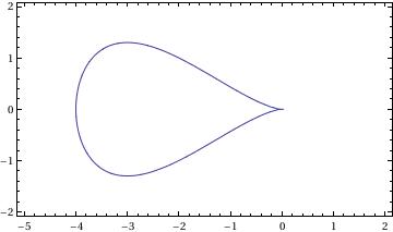
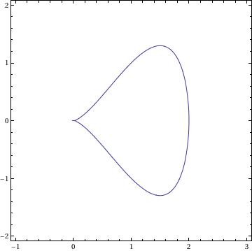
Antiversiera
For two values of parameters:
a=-2; b=1;
and
a = 1; b = 2;
we have two graphs:
ContourPlot[ x^4 - 2*a*x^3 + 4*a^2/b^2*y^2 == 0, {x, -5, 2}, {y, -2, 2}, AspectRatio -> Automatic]
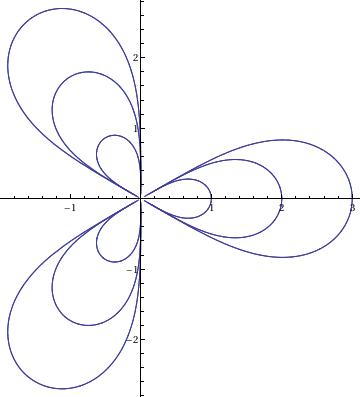
Arachnida
a = 1; n = 3;
PolarPlot[ 2*a*Sin[n*\[Phi]]/Sin[(n - 1)*\[Phi]], {\[Phi], .0001, 2*\[Pi]}]
PolarPlot[ 2*a*Sin[n*\[Phi]]/Sin[(n - 1)*\[Phi]], {\[Phi], .0001, 2*\[Pi]}]
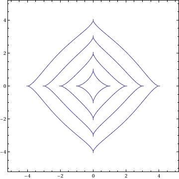
Astroid
t = {1, 2, 3, 4};
ContourPlot[(x^2 + y^2 - t^2)^3 + 27*x^2*y^2 == 0, {x, -5, 5}, {y, -5, 5}]
or
ContourPlot[(x^2 + y^2 - t^2)^3 + 27*x^2*y^2 == 0, {x, -5, 5}, {y, -5, 5}]
ContourPlot[x^(2/3) + y^(2/3) = 1, {x,-1,1},{y,-1,1}]
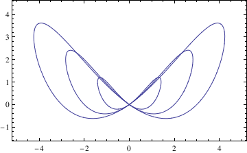
Besace
a = {1, 2, 3}; b = {1, 2, 3};
ContourPlot[(x^2 - b*y)^2 + a^2*(y^2 - x^2) == 0, {x, -5, 5}, {y, -1.5, 4.5}, AspectRatio -> Automatic]
ContourPlot[(x^2 - b*y)^2 + a^2*(y^2 - x^2) == 0, {x, -5, 5}, {y, -1.5, 4.5}, AspectRatio -> Automatic]
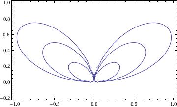
Bifolium
b = {0, 1, 2, 3};
ContourPlot[(x^2 + y^2)^2 == b*x^2*y, {x, -1, 1}, {y, -0.2, 1}, AspectRatio -> Automatic]
ContourPlot[(x^2 + y^2)^2 == b*x^2*y, {x, -1, 1}, {y, -0.2, 1}, AspectRatio -> Automatic]
Cardioid
r = {1, 2, 3};
PolarPlot[2*r*(1 - Cos[\[Phi]]), {\[Phi], 0, 2*\[Pi]}, AspectRatio -> Automatic]
PolarPlot[2*r*(1 - Cos[\[Phi]]), {\[Phi], 0, 2*\[Pi]}, AspectRatio -> Automatic]
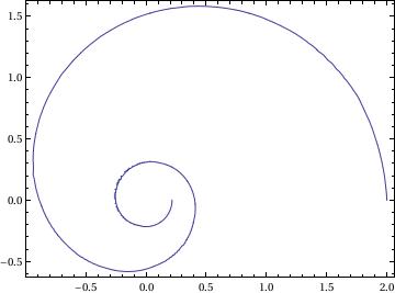
Circular Tractrix
a:=1;
f[r_, th_] := th - ArcTan[Sqrt[4*a^2 - r^2]/r] - Sqrt[4*a^2 - r^2]/r
g[r_, th_] := {r Cos[th], r Sin[th]}
pl = ContourPlot[f[r, th] == 0, {r, 0, 8 Pi}, {th, 0, 4 Pi}, PlotPoints -> 30];
pl[[1, 1]] = g @@@ pl[[1, 1]];
Show[pl, PlotRange -> All, AspectRatio -> 1.5/2]
f[r_, th_] := th - ArcTan[Sqrt[4*a^2 - r^2]/r] - Sqrt[4*a^2 - r^2]/r
g[r_, th_] := {r Cos[th], r Sin[th]}
pl = ContourPlot[f[r, th] == 0, {r, 0, 8 Pi}, {th, 0, 4 Pi}, PlotPoints -> 30];
pl[[1, 1]] = g @@@ pl[[1, 1]];
Show[pl, PlotRange -> All, AspectRatio -> 1.5/2]
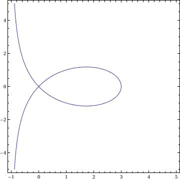
Cramer
r=2;l=1;
ContourPlot[ x*(x^2 + y^2) == (r + l)*x^2 - (r - l)*y^2, {x, -1, 5}, {y, -5, 5}, AspectRatio -> 1]
ContourPlot[ x*(x^2 + y^2) == (r + l)*x^2 - (r - l)*y^2, {x, -1, 5}, {y, -5, 5}, AspectRatio -> 1]
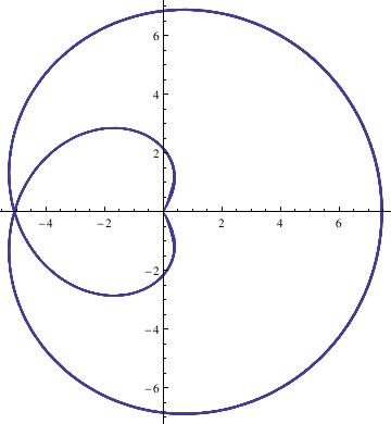
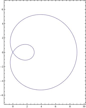
Epicycloid
R = 1; h = 5; r = 2;
PolarPlot[Sqrt[ R^2 + h^2 - 2*(R + r)*h*Cos[R/r*\[Phi]]], {\[Phi], 0, 200*\[Pi]}]
PolarPlot[Sqrt[ R^2 + h^2 - 2*(R + r)*h*Cos[R/r*\[Phi]]], {\[Phi], 0, 200*\[Pi]}]
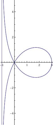
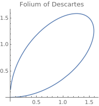
Folium of Descartes
Clear[f, g, t];
f[t_] = 3 t/(1 + t^3);
g[t_] = 3 t^2 /(1 + t^3);
ParametricPlot[{f[t], g[t]}, {t, 0, 20}, PlotRange ->All, AspectRatio -> 1, Plotlabel -> "Folium of Descartes", ImageSize ->200]
g[t_] = 3 t^2 /(1 + t^3);
ParametricPlot[{f[t], g[t]}, {t, 0, 20}, PlotRange ->All, AspectRatio -> 1, Plotlabel -> "Folium of Descartes", ImageSize ->200]
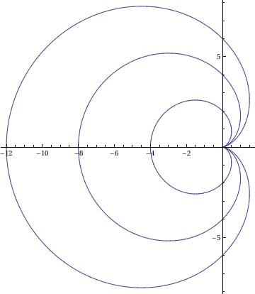
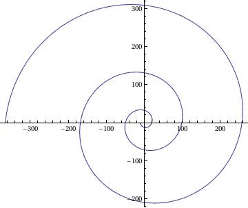
Galileo's Spiral
a=-1;l=10;
PolarPlot[a*\[Phi]^2 - l, {\[Phi], 0, 6*\[Pi]}]
PolarPlot[a*\[Phi]^2 - l, {\[Phi], 0, 6*\[Pi]}]
Kiepert
|
l = {1, 2, 3};
PolarPlot[(l^3*Cos[3*\[Phi]])^(1/3), {\[Phi], -2*\[Pi], 2*\[Pi]} |
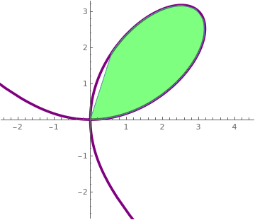
Lemniscate
|
F[t_] := 6*(Sec[t] Tan[t])/(1 +Tan[t]^3)
lemniscate = PolarPlot[F[t], {t,-Pi/6, 3*Pi/4.2}, PlotStyle -> {{Purple, Thickness[0.01]}}] ; shadingRight = ParametricPlot[{F[t]}, {t,0,CubeRoot[2]}, {r,0,F[t]}, PlotStyle -> {Red, Opacity[0.5]}, Mesh->None]; shadingLeft = ParametricPlot[{r*Cos[t], r*Sin[t]}, {t,0,CubeRoot[2]}, {r,0,F[t]}, PlotStyle -> {Green, Opacity[0.5]}, Mesh->None]; Show[lemniscate,shadingRight,shadingLeft] |
Limaçon
|
a=3; l=3;
ContourPlot[(x^2 + y^2 - 2*a*x)^2 == l^2*(x^2 + y^2), {x, -1, 10}, {y, -7, 7}, AspectRatio -> 14/11] |
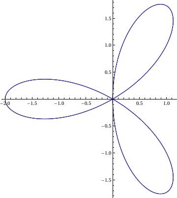
Rose
k=3;
PolarPlot[a*Cos[k*\[Phi]], {\[Phi], 0, 4*\[Pi]}]
PolarPlot[a*Cos[k*\[Phi]], {\[Phi], 0, 4*\[Pi]}]
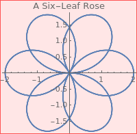
PolarPlot[2 Cos[3*theta/2], {theta, -4*Pi, 4*Pi}, PlotLabel ->"A Six-Leaf Rose", AspectRatio ->Automatics, ImageSize->200]
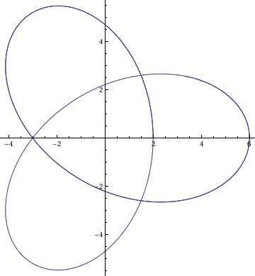
Trefoil
r=2;
ParametricPlot[{r*(2*Cos[2*t] - Cos[t]), r*(2*Sin[2*t] + Sin[t])}, {t, 0, 10}]
ParametricPlot[{r*(2*Cos[2*t] - Cos[t]), r*(2*Sin[2*t] + Sin[t])}, {t, 0, 10}]
Return to Mathematica page
Return to the main page (APMA0330)
Return to the Part 1 (Plotting)
Return to the Part 2 (First Order ODEs)
Return to the Part 3 (Numerical Methods)
Return to the Part 4 (Second and Higher Order ODEs)
Return to the Part 5 (Series and Recurrences)
Return to the Part 6 (Laplace Transform)
Return to the Part 7 (Boundary Value Problems)