Return to computing page for the first course APMA0330
Return to computing page for the second course APMA0340
Return to computing page for the fourth course APMA0360
Return to Mathematica tutorial for the first course APMA0330
Return to Mathematica tutorial for the second course APMA0340
Return to Mathematica tutorial for the fourth course APMA0360
Return to the main page for the course APMA0330
Return to the main page for the course APMA0340
Return to the main page for the course APMA0360
Return to Part II of the course APMA0330

Preface


A null-space (also called kernel) of the first order differential operator could have a very complicated structure. A one-dimensional set of functions that depends continuously on one parameter is called the general solution if every element of it is annihilated by the operator. When it has besides a one-dimensional space some other elements, then a corresponding initial value problem has multiple solutions and uniqueness fails. This case is not suitable for computer applications. Here, an initial value problem has a solution that cannot be obtained from the general solution by choosing an appropriate value of an arbitrary constant. Such a solution is called a singular solution.

Singular Solutions


Consider a first order differential equation
\begin{equation} \label{EqSingular.1} F\left( x, y , y' \right) =0, \qquad \mbox{where} \quad y' = {\text d}y/{\text d}x = {\texttt D}y \end{equation}
is the derivative of the function y(x) with respect to independent variable x. If the function F is smooth, then Eq.\eqref{EqSingular.1} can be solved with respect to y' according to the inverse function theorem; this leads to the differential equation in the normal form:
\begin{equation} y' = f(x,y) \qquad\mbox{or in operator form}\qquad F[y] = \texttt{D}\,y - f(x,y) = 0. \label{EqSingular.2} \end{equation}
Solving Eq.\eqref{EqSingular.1} is equivalent to determining of the null-space (also called kernel) of the operator F. Generally speaking, F is an operator because it assigns to every input function y(x) the output F[y], involving a derivative operator \( \texttt{D} = {\text d}/{\text d}x . \) By solving Eq.\eqref{EqSingular.1}, one determines every function y(x) that is annihilated by the operator F(x, y, y') or F[y]. For differential operator \eqref{EqSingular.2} to be applied to function y(x), this function must have a continuous derivative; this situation is usually abbreviated as y ∈ ℭ¹ or yC¹. We know from calculus that \( \texttt{D} \) is an unbounded operator and its null-space is a one dimensional space spanned on the constant function y(x) = c. We also know that \( \texttt{D}^{-1} \,f(x) = \int f(x) \,{\text d} x + c . \) Note that D-1 is not a true inverse, but only the right inverse: \( \texttt{D}\,\texttt{D}^{-1} = I , \) where I is the identical operator. To see why \( \quad \texttt{D}^{-1} \texttt{D} \ne I, \) compute
\[ \texttt{D}^{-1} \texttt{D}\, f(x) = \texttt{D}^{-1} f' (x) = \int f' (x)\,{\text d} x + c = f(x) + c . \]
Therefore, it is expected that the null-space of F is also a one-dimensional space depending on some constant. If this is true, the null-space is called the general solution unlike in calculus where the term «antiderivative» is used. A general solution of Eq.\eqref{EqSingular.1} or \eqref{EqSingular.2} depends on a constant and is usually written as a relation
\begin{equation} \psi (x, y, c ) = 0 , \label{EqSingular.3} \end{equation}
where c is an arbitrary constant from some domain. Equation \eqref{EqSingular.3} defines a one-parameter family of solutions to the equation F(x, y, y') = 0. However, for some equations, the null-space of F(x, y, y') = 0 is more complicated and may contain functions that are not included in the general form: such solutions deserve special attention. The differential equation \eqref{EqSingular.1} may have solutions that cannot be obtained from ψ(x, y, c) = 0 for an appropriate choice of the constant c.
A solution is called the singular solution of the differential equation F(x, y, y') = 0 if it cannot be obtained from the general solution for any choice of arbitrary constant c, including infinity. In other words, if the initial value problem has at least two solutions, then those of which that is not a member of the general solution is called singular.
Therefore, the null-space of the differential operator \eqref{EqSingular.1} may consist of two parts: solutions that are determined by the relation \eqref{EqSingular.3} (called the general solution) and those that are not identified by Eq.\eqref{EqSingular.3}. The latter comprises the set of singular solutions. Uniqueness theorems, presented in section, show the cases when singular solutions do not exist. For example, if a slope function in Eq.\eqref{EqSingular.2} is a Lipschitz function in variable y, then a singular solution does not exist. You will learn later that linear equations as well and Bernoulli equations have no singular solutions.

Obviously, an initial value problem with multiple solutions may be not suitable for modeling because it confuses the software in use. In applications, when uniqueness of solutions is required, singular solutions must be eliminated.

One of the common ways to determine existence of a singular solution is to eliminate c from the system of equations:

\[ \psi \left( x, y, c \right) =0 , \qquad \frac{\partial \psi}{\partial c} = 0. \]
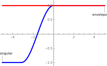
A singular solution in a stronger sense is such function that is tangent to every solution from a family of solutions, forming the envelope of this family of solutions.

Constant functions are usually not solutions of the differential equations unless they annihilate the slope function. In this case, we call them critical points or equilibrium/stationary solutions. Therefore, if y = y* vanishes the slope function, \( f(x, y^{\ast} ) \equiv 0 , \) then y = y* is the equilibrium solution of the differential equation \( y' = f(x, y ) . \) A stationary solution may be singular or not, which we will show in the following examples.

Example 1: 
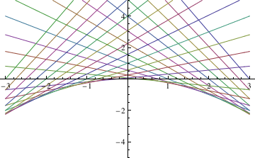
Consider Clairaut's equation
y=xy' + (y')^2
Clear[y];
y[x_] = x c + c^2
samples =Table[y[x],{c,-3,3,1/4}]
Plot[Evaluate[samples],{x,-3,3},PlotRange->{-5,5}]
Out[18]= c^2 + c x
Out[19]= {9 - 3 x, 121/16 - (11 x)/4, 25/4 - (5 x)/2, 81/16 - (9 x)/4, 4 - 2 x,
49/16 - (7 x)/4, 9/4 - (3 x)/2, 25/16 - (5 x)/4, 1 - x,
9/16 - (3 x)/4, 1/4 - x/2, 1/16 - x/4, 0, 1/16 + x/4, 1/4 + x/2,
9/16 + (3 x)/4, 1 + x, 25/16 + (5 x)/4, 9/4 + (3 x)/2,
49/16 + (7 x)/4, 4 + 2 x, 81/16 + (9 x)/4, 25/4 + (5 x)/2, 121/16 + (11 x)/4, 9 + 3 x}
Out[20]=

To find the singular solution (envelope), we type:

f[t_] = t^2;
Eliminate[{x==-f'[t],y==f[t]-t*f'[t]},t]
Out[37]= -4y==x^2

   ■
Example 2: Consider the generalized Clairaut equation
\[ \left( x y' -y \right)^2 = 4\left( y' \right)^2 , %y' \left( x\,y' -3\,y \right) + 2 = 0 . \tag{2.1} \]
This generalized Clairaut equation unites two separable equations
\[ y' = \frac{y}{x-2} \qquad \mbox{and} \qquad y' = \frac{y}{x+2} , \qquad x\ne \pm 2. \tag{2.2} \]
Solve[(x*p - y)^2 == 4*p^2, p]
{{p -> y/(-2 + x)}, {p -> y/(2 + x)}}
Equations (2.2) have general solutions:
\[ y = \left( x- 2 \right) c_1 \qquad \mbox{and} \qquad y = \left( x+ 2 \right) c_2 , \tag{2.3} \]
that depend ontwo arbitrary constants c₁ and c₂. The general solution of Generalized Clairaut equation (2.1) is
\[ \left( x \,C -y \right)^2 = 4\,C^2 \qquad \Longrightarrow \qquad y = C\left( x \pm 2 \right) , \tag{2.4} \]
where C is a constant. Differentiating with respect to C, we get two singula solutions
\[ x\pm 2 = 0 \tag{2.5} \]
These two envelopes of singular solutions (2.5) separate the plane (x, y) ∈ ℝ² into three domains filled with members of the general solutions (2.3).
      Now we plot some representatives from the general solution.
plot=Plot[{Callout[x + 2, "c=1", Above, Frame -> True, FrameMargins -> 10], Callout[2*x + 2, "c=2", Below, Frame -> True, CalloutStyle -> Yellow], Callout[3*x - 6, "c=3", Right, Frame -> True, Background -> Pink], Callout[-2*x + 4, "c=-2", Right, Frame -> True, Background -> LightBlue], Callout[-3*x + 6, "c=-3", Right, Frame -> True, Background -> LightBlue]}, {x, -5, 5}, PlotStyle -> Thickness[0.01]];
line1 = Graphics[{Dashed, Red, Thickness[0.01], Line[{{2, -5}, {2, 9}}]}];
line2 = Graphics[{Dashed, Red, Thickness[0.01], Line[{{-2, -5}, {-2, 9}}]}];
line2a = Graphics[{Dashed, Red, Thickness[0.01], Line[{{-2, 9}, {-2, 19}}]}];
line2b = Graphics[{Dashed, Red, Thickness[0.01], Line[{{-2, -5}, {-2, -19}}]}];
Show[line1, line2, line2a, line2b, plot, AspectRatio -> 0.9]
       The family of solutions and two singular solutions x = ±2.            Mathematica code

   ■
Example 3: Consider the autonomous equation
\[ \frac{{\text d}y}{{\text d}x} = \sqrt{1-y^2} \qquad (y^2 \le 1). \]
Separation of variables and integration yields
\[ \frac{{\text d}y}{\sqrt{1-y^2}} = {\text d}x \Longrightarrow \qquad \arcsin y = x + c , \]
where c is a constant of integration. For y ∈ [-1, 1], we apply sine function and obtain
     
y1[x_] = Piecewise[{{0, x < -Pi/2}, {Sin[x], -Pi/2 <= x <= Pi/2}, {0, x > Pi/2}}];
y2[x_] = Piecewise[{{0, x < -Pi/2 - 1.5}, {Sin[x + 1.5], -Pi - 1.5/2 <= x <= Pi/2 - 1.5}, {0, x > Pi/2 - 1.5}}];
y3[x_] = Piecewise[{{0, x < -Pi/2 + 2.5}, {Sin[x - 2.5], -Pi + 2.5/2 <= x <= Pi/2 + 2.5}, {0, x > Pi/2 + 2.5}}];
Plot[{Callout[y1[x], "c=0", Above], Callout[y2[x], "c=-1.5", Below], Callout[y3[x], "c=2.5", Above]}, {x, -5, 5}, PlotStyle -> Thickness[0.01]]
       Three members of the general solution.            Mathematica code

One of these curves from the primitive F(x, y, y') = 0 can be chosen to satisfy the initial condition y(x0) = y0:
\[ x - x_0 = \arcsin y - \arcsin y_0 \qquad -1 \le y \le 1 , \quad -1 - \arcsin y_0 \le x - x_0 \le 1 - \arcsin y_0 . \]
However, the given initial value problem:
\[ y' = \sqrt{1-y^2} , \qquad y\left( x_0 \right) = 1 \]
has a singular solution:
\[ y(x) = \begin{cases} 1, & \ \mbox{ for } x > x_0 , \\ \cos \left( x - x_0 \right) , & \ \mbox{ for } x_0 - \pi < x < x_0 , \\ -1 , & \ \mbox{ for } x < x_0 - \pi . \end{cases} \]
      Now we plot the singular solution (in blue) along with the singular envelope (in red).
s[x_] = Piecewise[{{1, x > 0}, {Cos[x], -Pi <= x <= 0}, {-1, x < -Pi}}];
env[x_] = 1;
Plot[{Callout[s[x], "singular", Left], Callout[env[x], "envelope", Right]}, {x, -5, 5}, PlotStyle -> {{Blue, Thickness[0.01]}, {Red, Thickness[0.01]}}]
       Singular solution and the envelope.            Mathematica code

The equilibrium solution y = 1 is a singular envelope for the family of general solutions.    ■
Example 4: Consider the initial value problem
\[ \frac{{\text d}y}{{\text d}x} = \begin{cases} \frac{4 x^3 y}{x^4 + y^2}, & \ \mbox{ if } x \ne 0 \quad\mbox{or}\quad y \ne 0, \\ 0, & \ \mbox{ if } x=y=0 . \end{cases} \qquad y(0) = 0. \]
It is easy to show that the slope function, which we denote by f(x, y), is a continuous function in two variables x and y. On the other hand,
\[ \left\vert f(x, y_1 ) - f(x, y_2 ) \right\vert = \left\vert \frac{4 x^3 y_1}{x^4 + y^2_1} - \frac{4 x^3 y_2}{x^4 + y^2_2} \right\vert = \frac{4 x^3 \left( x^4 - y_1 y_2 \right)}{\left( x^4 + y_1^2 \right)\left( x^4 + y_2^2 \right)} \left( y_2 - y_1 \right) . \]
If y1 = px² and y2 = qx², then
\[ \left\vert f(x, y_1 ) - f(x, y_2 ) \right\vert = 4\left\vert \frac{1-pq}{\left( 1 + p^2 \right)\left( 1 + q^2 \right)} \right\vert \left\vert \frac{y_2 - y_1}{x} \right\vert . \]
Therefore, the Lipschitz condition is not satisfied throughout any region containing the origin.

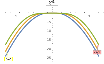
The given equation admits the explicit solution

\[ y = c^2 - \sqrt{x^4 + c^2} , \]
containing an arbitrary real constant c. Since this function satisfies the initial condition y(0) = 0, the given initial value problem has infinite many solutions.
      Now we plot several singular solutions.
Plot[{Callout[(x + 2)/3, "c=1", Left, Frame -> True, FrameMargins -> 10], Callout[(4*x + 2)/6, "c=2", Below, Frame -> True, CalloutStyle -> Yellow], Callout[(9*x + 2)/9, "c=3", Right, Frame -> True, Background -> Pink], Callout[(4*x + 2)/(-6), "c=-2", Right, Frame -> True, Background -> LightBlue]}, {x, -5, 5}, PlotStyle -> Thickness[0.01]]
       Three singular solutions.            Mathematica code

   ■


  1. Coddington, E.A. and Levinson, N., Theory of Ordinary Differential Equations, ‎ McGraw-Hill; 1st edition, 1984.
  2. Dobrushkin, V.A., Applied Differential Equations: The Primary Course, Second edition, CRC Press, Boca Raton, FL, 2022.
  3. Hale, J.K., Ordinary Differential Equations (Dover Books on Mathematics), Illustrated Edition, 2009.
  4. Ince, E.L., Ordinary Differential Equations (Dover Books on Mathematics) Illustrated Edition, 1956.


Return to Mathematica page
Return to the main page (APMA0330)
Return to the Part 1 (Plotting)
Return to the Part 2 (First Order ODEs)
Return to the Part 3 (Numerical Methods)
Return to the Part 4 (Second and Higher Order ODEs)
Return to the Part 5 (Series and Recurrences)
Return to the Part 6 (Laplace Transform)
Return to the Part 7 (Boundary Value Problems)