Preface
This section is devoted to a review of the basic terminology and definitions of solutions to differential equations. Since this topic becomes a substantial part of functional analysis and operator theory, this section also addresses this point of view in layman's terms.
Return to computing page for the second course APMA0340
Return to Mathematica tutorial for the first course APMA0330
Return to Mathematica tutorial for the second course APMA0340
Return to the main page for the course APMA0330
Return to the main page for the course APMA0340
Glossary
Solutions to ODEs
The first order differential equation \( R(x,y,y' ) = 0 \) is an equation containing a derivative of an unknown function. It can be also written in the equivalent form involving differentials \( G \left( x,y,{\text d}x. {\text d}y \right) = 0 . \) The derivative of any function is the result of applying the derivative operator to the function. This can usually be denoted by using Euler's notation \( \texttt{D} = {\text d}/{\text d}x , \) which is an unbounded (not continuous) operator because it may map a bounded function into unbounded one. The operator D does not act on arbitrary functions, such as the absolute value function. The function must be smooth so that the derivative operator can be applied. The derivative operator is defined on some subset of continuous functions. So, the domain of the derivative operator includes only continuously differential functions on some open interval (𝑎,b) that we denote as C¹(𝑎,b) or simply C¹. Because D is unbounded, every differential equation should be considered on a set of functions that have a continuous derivative on some open interval.
In calculus, you learn that the simplest differential equation Dy = f(x) has infinitely many solutions \( y(x) = \int f(x)\,{\text d}x +c , \) depending on an arbitrary constant c, because the derivative operator D annihilates constants. So the null-space of the derivative operator is a one-dimensional space spanned on any nonzero constant function. (Remember: the derivative of any constant, regardless of its value, will always be zero.) For example, the differential equation y' = x-1 has the solution \( y(x) = \int x^{-1}\,{\text d}x + c = \ln |x| + c, \) where c is any real constant. However, we can represent this constant as logarithm c = lnC, where C is some positive number. Then our solution becomes \( y(x) = \ln (c\,|x|) = \ln C\,x , \) where C is a positive constant when x is positive and C becomes negative for negative independent variable x. Therefore, in our formula, C is an arbitrary constant, but taking from some domain depending on the independent variable. This example shows that an arbitrary constant that is used to represent a solution of a differential equation should be chosen with care from some domain depending on the formula in use.
Now we discuss a topic of inverse differential operators that we started previously in the section. This means that the inverse operator D-1 does not exist and the domain of D must be more restricted in order to find its inverse. Therefore, you expect that a first order differential equation also has infinitely many solutions depending on an arbitrary constant. It turns out that this is usually the case (with some exceptions), but an arbitrary constant C is not 100% arbitrary and should be taken from some domain depending on the problem and its possible solution. It is a custom to call such family of solutions depending on a constant, the general solution, leaving the word antiderivative to calculus.
|
> > > |
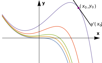
DSolve[{y'[x] == y[x] - x^2, y[0] == a}, y[x], x] f[a_, x_] = 2 - 2 E^x + a E^x + 2 x + x^2; parameters = {0, 0.1, 0.2, 0.5, 1}; family = Plot[Evaluate[f[#, x] & /@ parameters], {x, -2, 3.3}, PlotRange -> {-2, 3}, Axes -> False]; a1 = Graphics[{Black, Arrowheads[0.06], Arrow[{{-2, 0}, {3.3, 0}}]}]; a2 = Graphics[{Black, Arrowheads[0.06], Arrow[{{0, -2}, {0, 3}}]}]; ll = Graphics[{Thick, Line[{{1.85, 3}, {2.8, 1.0}}]}]; p = Graphics[{PointSize[Large], Purple, Point[{2.13, 2.38}]}]; t1 = Graphics[ Text[StyleForm["(" Subscript[x, 0], FontSize -> 14], {2.4, 2.5}]]; t1a = Graphics[Text[StyleForm[",", FontSize -> 16], {2.66, 2.5}]]; t1b = Graphics[ Text[StyleForm[Subscript[y, 0], FontSize -> 14], {2.84, 2.5}]]; t1c = Graphics[Text[StyleForm[")", FontSize -> 14], {3.05, 2.5}]]; t2 = Graphics[ Text[StyleForm["y'(" Subscript[x, 0], FontSize -> 14], {3.1, 1.1}]]; t2a = Graphics[Text[StyleForm[")", FontSize -> 14], {3.39, 1.1}]]; tx = Graphics[ Text[StyleForm["x", FontSize -> 14, FontWeight -> "Bold"], {3.2, 0.35}]]; ty = Graphics[ Text[StyleForm["y", FontSize -> 14, FontWeight -> "Bold"], {0.25, 2.75}]]; Show[family, a1, a2, ll, p, t1, t1a, t1b, t1c, t2, t2a, tx, ty] |
The situation is similar to some practical problems from physics and mechanics. Suppose we have a single railcar (engine) moving along a track that we can describe by the function x(t). If we express its velocity as a function of time and position, we get the first order differential equation \( v = \dot{x} = f(t,x) , \) where x is a position of the engine at time t. Its position x(t) has one degree of freedom because the location of the car is defined by the distance along the track.
Suppose we want to find a solution that satisfies the initial condition y(0) = -1. This leads to the equation \( e^c = -1 , \) that tells us that \( c = {\bf j}\pi + 2k\,{\bf j}\pi , \) for k = 0, ±1, ±2, … , where j is the unit vector in the positive direction on the complex plane ℂ. Although the given initial value problem has a unique solution, it has infinitely many ways to write it down. Therefore, representing the family of solutions in the form \( y = e^{x+c} \) yields complex choice for an arbitrary constant c.
Our next differential equation
Since the general solution of the differential equation is usually not possible to determine, we need a way to pin down a particular solution. The most obvious possibility to identify a particular solution is to impose the initial condition by specifying the value of a solution at some point. The corresponding problem, which is called the initial value problem, consists of some differential equation together with an initial condition:
Members of the family of solutions that form the general solution do not intersect and do not touch each other. Why? If two members of the general solution will have a common point, then at this point we would have two solutions of the same equation written in implicit form. However, there could be other solutions that may touch some members of the general solution. These exceptional solutions are called singular solutions.
General Solution
It is expected that we observe a similar property in general case of Eq.\eqref{EqSolution.1}. Unfortunately, in this case the null-space of the inverse operator \( \texttt{D}^{-1} \) applied to function f(x, y) may be more complicated than just one dimensional space. Therefore, in the theory of differential equation the word antiderivative is not used because it does not reflect the general situation. Instead, we use expression general solution that means a one-dimensional subspace of the null-space \( \texttt{D}^{-1} f(x,y) . \)
Let us look at formation of the differential equation from another prospective. Suppose we are given a one-dimensional family of smooth functions F(x, y, c) = 0, where c is a real parameter. Upon differentiating this relation we get
|
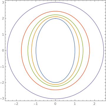
parameters = {0, 0.5, 1.0, 2.05, 5.1};;
ContourPlot[ Evaluate[f[x, y, #] == 1 & /@ parameters], {x, -2.5, 2.5}, {y, -4, ; 4}, AspectRatio -> 1, PlotRange -> {-2, 2}, ; PlotLegends -> Table[Row[{"c=", j}], {j, parameters}]] |
|
| Confocal conics. | Mathematica code |
The differential equation that is primitive is obtained by eliminating c between it and the derivative equation
We can conclude that a family of curves depending on n parameters generates a differential equation for which this family provides a general solution. However, it is not evident that any differential equation of order n can be derived from such primitive. It does not follow that if the differential equation is given, it possesses a general solution that depends upon n arbitrary constants. This conclusion follows from the existence and uniqueness theorem that guarantees dependence of the general solution on n initial conditions. In the formation of a differential equation from a given family of integral curves, corresponding conditions must be assumed to be satisfied as it is required by the existence theorem. The role of n arbitrary constants can play n initial conditions---they are more natural than finding a corresponding primitive (= implicit general solution). You will learn shortly that such general solution is impossible to construct explicitly for an arbitrary differential equation even if it is known that the corresponding primitive exists.
From a theoretical point of view, a differential equation can be considered as an unbounded operator (because it contains a derivative operator) mapping a smooth function into another continuous function. Its null-space is at least n-dimensional, which is reflected by the general solution containing exactly n arbitrary constants. Therefore, a general solution of any differential equation of order n should contain exactly n arbitrary constants taken from some domain (assuming that the equation has a solution). Does it mean that any solution to the differential equation should be a member of the general solution? The answer is negative because some nonlinear differential equations may have solutions not included in the general solution. We will discuss these exceptional solutions, called the singular solutions in the next section.
Solution terminology
| Term | Meaning | Example |
|---|---|---|
| solution family | a family of functions or relations, with one or more parameters possibly subject to some constraints, such that for every choice of parameter values subject to those constraints, we get a particular solution. | \( y = \cosh (x + C) \) with parameter C ∈ ℝ, is a solution family for \( y^2 - (y' )^2 =1 . \) |
| general solution | a family of solutions including a one-dimensional subspace of the null-space depending on one arbitrary constant; it covers almost all solutions excluding some exceptions | The general solution to \( y' = 1 \) is \( y = x + C , \) where C ∈ ℝ. |
| explicit solution | a solution of the differential equation that is expressed as some known function y = φ(x). | \( y = 2 \left( C - x^2 \right)^{-1} \) is an explicit (general) solution to the differential equation \( y' = x\,y^2 . \) | implicit solution | a solution of the differential equation in the form f(x,y) = 0 for some function f that does not depend on the derivative. | \( 2 = y \left( C - x^2 \right) \) is an implicit (general) solution to the differential equation \( y' = x\,y^2 . \) | particular solution | a function or relation that defines a solution for the differential equation. Usually,a particular solution is obtained from the general solution by choosing a particular value for the parameter of from the initial value problem. | y = cosh x is a functional solution to \( y^2 - (y' )^2 =1 . \) |
| singular solution | a solution of the differential equation that cannot be obtained from the general solution for any values of constant C, including infinity, and for which the initial value problem has multiple solutions. | y ≡ 0 is a singular solution to the initial value problem \( y' = \sqrt{y}, \ y(0) =0 . \) |
| solution to initial value problem | a particular solution that satisfies the initial value condition. | A particular solution to \( y' + y = 1, \ y(0) =2 \) is \( y = 1 + e^{-x} . \) |
Constant functions are usually not solutions of the differential equations unless they annihilate the slope function. In this case, we call them critical points or equilibrium/stationary solutions. Therefore, if y = y* vanishes the slope function, \( f(x, y^{\ast} ) \equiv 0 , \) then y = y* is the equilibrium solution of the differential equation \( y' = f(x, y ) . \) A stationary solution may be singular or not, which we will show in the following examples in the next section.
- Bougoffa, L., On the exact solutions for initial value problems of second-order differential equations, Applied Mathematics Letters, 2009, Vol. 22, pp. 1248--1251.
- Hasan, Y.Q., A new development to the Adomian decomposition for solving singular IVP of Lane--Emden type, United States of America Research Journal (USARJ), 2014, Vol. 2, No.3, pp. 9--13.
Return to Mathematica page
Return to the main page (APMA0330)
Return to the Part 1 (Plotting)
Return to the Part 2 (First Order ODEs)
Return to the Part 3 (Numerical Methods)
Return to the Part 4 (Second and Higher Order ODEs)
Return to the Part 5 (Series and Recurrences)
Return to the Part 6 (Laplace Transform)
Return to the Part 7 (Boundary Value Problems)