A Bernoulli differential equation is an equation of the form \( y' + a(x)\,y = g(x)\,y^{\nu} , \) where a(x) are g(x)
are given functions, and the constant ν is assumed to be any real number other than 0 or 1. It is an example of a non-linear differential equation for which a general solution can be obtained in closed form.
Bernoulli equations have no singular solutions.
The Wolfram Mathematica notebook that contains the code that produces all the Mathematica outputs in this web page may be downloaded at this link.
Return to computing page for the first course APMA0330
Return to computing page for the second course APMA0340
Return to Mathematica tutorial for the first course APMA0330
Return to Mathematica tutorial for the second course APMA0340
Return to Mathematica tutorial for the third course APMA0360
Return to the main page for the course APMA0330
Return to the main page for the course APMA0340
Return to the main page for the course APMA0360
Return to Part II of the course APMA0330
where α is a real number not equal to 0 or 1, is called a Bernoulli differential equation. It is named after Jacob (also known as James or Jacques)
Bernoulli (1654--1705) who discussed it in 1695. Jacob Bernoulli was born in Basel, Switzerland. Following his
father's wish, he studied theology and entered the ministry. But contrary to the desires of his parents, he also
studied mathematics and astronomy. He traveled throughout Europe from 1676 to 1682, learning about the latest
discoveries in mathematics and the sciences under leading figures of the time. His travels allowed him to establish
correspondence with many leading mathematicians and scientists of his era, which he maintained throughout his life.
Bernoulli returned to Switzerland and began teaching mechanics at the University in Basel from 1683. In 1684 he
married Judith Stupanus. They had two children. He was appointed professor of mathematics at the University of
Basel in 1687, remaining in this position for the rest of his life. By that time, he had begun tutoring his younger brother
Johann Bernoulli on mathematical topics. The two brothers began to study the calculus as presented by Leibniz in his
1684 paper on the differential calculus. Jacob collaborated with his brother on various applications of calculus.
However the atmosphere of collaboration between the two brothers turned into rivalry as Johann's own mathematical
genius began to mature, with both of them attacking each other in print, and posing difficult mathematical
challenges to test each other's skills. By 1697, the relationship had completely broken down.
Jacob Bernoulli is known for his numerous contributions to calculus, and along with his brother Johann, was one
of the founders of the calculus of variations. In May 1690, in a paper published in Acta Eruditorum, Jacob Bernoulli
showed that the problem of determining the isochrone is equivalent to solving a first-order nonlinear differential
equation. The isochrone, or curve of constant descent, is the curve along which a particle will descend under
gravity from any point to the bottom in exactly the same time, no matter what the starting point. He also discovered
the fundamental mathematical constant e, which Euler later denoted by e.
Jacob made a great contribution to calculus. By 1689 he had published important work on infinite series and showed
that harmonic series diverges, which had actually been proved by Mengoli 40 years earlier. Jacob Bernoulli also
discovered a general method to determine evolutes of a curve as the envelope of its circles of curvature. He also
investigated caustic curves and in particular he studied these associated curves of the parabola, the logarithmic
spiral and epicycloids around 1692. The lemniscate of Bernoulli was first conceived by Jacob Bernoulli in 1694.
In 1695 he investigated the drawbridge problem which seeks the curve required so that a weight sliding along the
cable always keeps the drawbridge balanced.
However, his most important contribution was in the field of probability, where he derived the first version of
the law of large numbers in his work Ars Conjectandi, published in Basel in 1713, eight years after his death.
Jacob Bernoulli chose a figure of a logarithmic spiral (its equation in polar coordinates is
\( r = a\, e^{b\,\theta} \) ) and the motto Eadem mutata resurgo
("Changed and yet the same, I rise again") for his gravestone; the spiral executed by the stonemasons was,
however, an Archimedean spiral, \( r = a + b\, \theta . \)
Bernoulli equations are special because they are nonlinear differential equations with known exact solutions.
Moreover, they do not have singular solutions---similar to linear equations. There are two methods known to determine
its solutions: one was discovered by Bernoulli himself, and another is credited to
Gottfried
Leibniz (1646--1716).
Leibniz substitution
The Bernoulli equation \( \quad y' + p(x)\,y = g(x)\,y^\alpha \quad \) can be reduced to a linear
differential equation with substitution
The Bernoulli equation \( y' + p(x)\,y = g(x)\,y^\alpha \) can be reduced to two separable equations.
We seek its solution as the product of two functions \( y(x) = u(x)\,v(x) , \) where
u(x) is a solution (we need just one of them) of a linear part:
Example 1:
Consider the differential equation \( \quad
y\, y' = y^2 + e^x . \ \) Since in the given differential equation the derivative is not isolated, we divide both sides by y. As a result, we obtain a Bernoulli equation y′ = y + ex/y (here prime indicates differentiation: y′ = dy/dx). To solve it, we first use the Leibniz substitution: u = y². \( \displaystyle
\quad \Longleftrightarrow \quad y = u^{1/2} . \quad \) Then
\[
y' = \frac{1}{2}\, u^{-1/2} u'
\quad \Longrightarrow \quad y\,y' = \frac{1}{2}\, u'
\]
and we get the linear differential equation with respect to unknown function u:
\[
\frac{1}{2}\, u' = u + e^x .
\]
To solve it, we first find an integrating factor by solving the corresponding separable equation
where C is a constant of integration. Returning to the original function, we find the general solution to
the given differential equation \( y = \pm \sqrt{C\,e^{2x} - 2\, e^x} . \)
Now we demonstrate the application of the Bernoulli method by seeking the solution as the product y = u v,
where u is a solution of the "linear part:"
\[
u' = u \qquad \Longrightarrow \qquad u (x) = e^{x} .
\]
Then v must be the general solution to the separable equation
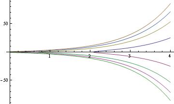
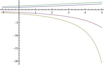
Example 2: The four streamlines (corresponding to the values of an arbitrary constant C=1,2,3,4) from the general solution y=1/(x Sqrt[C-2 ln[x]]) of the Bernoulli equation
x y' =x^2 y^3 -y can be plotted with one command:
Since \( y = u^{-1/3} , \) we obtain the general solution:
\[
y(x) = \left( 1 + C\, e^{3 x^2 /2} \right)^{-1/3} .
\]
We employ Mathematica to confirm our analytical manipulations. First, we define type in the Bernoulli equation and male Leibniz's substitution.
Now we find the general solution using the Bernoulli method: y = u·v, where u is a solution of the
"truncated" linear equation \( u' + x\,u =0 \) and v is the general solution of
the separable equation \( u\, v' = x\, \left( u\, v \right)^4 . \) Solving the equation
for u, we get
This answer is slightly different from the general solution obtained by Leibniz's method: it contains a multiple of "3" as a multiple of an arbitrary constant. Clearly, we can denote 3 c as a new constant, so both methods provide the same solutiuon.
■
End of Example 3
Example 4: (Logistic equation)
The logistic equation with harvesting \( \dot{y} = r\, y \left( 1 - \frac{y}{k} \right) - h\, y(t) \)
is an example of the Bernoulli equation. It is assumed that all coefficients (r, k, h) are constants. It
can be solved and plotted as follows.
LogisticEquation = y'[t] == r (1 - (y[t]/k))*y[t] - h*y[t];
DSolve[LogisticEquation, y, t]
Out[1]=
{{y -> Function[{t}, -((E^(r t + h k C[1]) k (-h + r))/(
E^(h t + k r C[1]) - E^(r t + h k C[1]) r))]}}
We define the solution function
sol = DSolve[{LogisticEquation /. {r -> (1/2), k -> 10, h -> (1/4)}, y[0] == a}, y, t]
Out[2]=
{{y -> Function[{t}, (5 a E^(t/4))/(5 - a + a E^(t/4))]}}
Example 5:
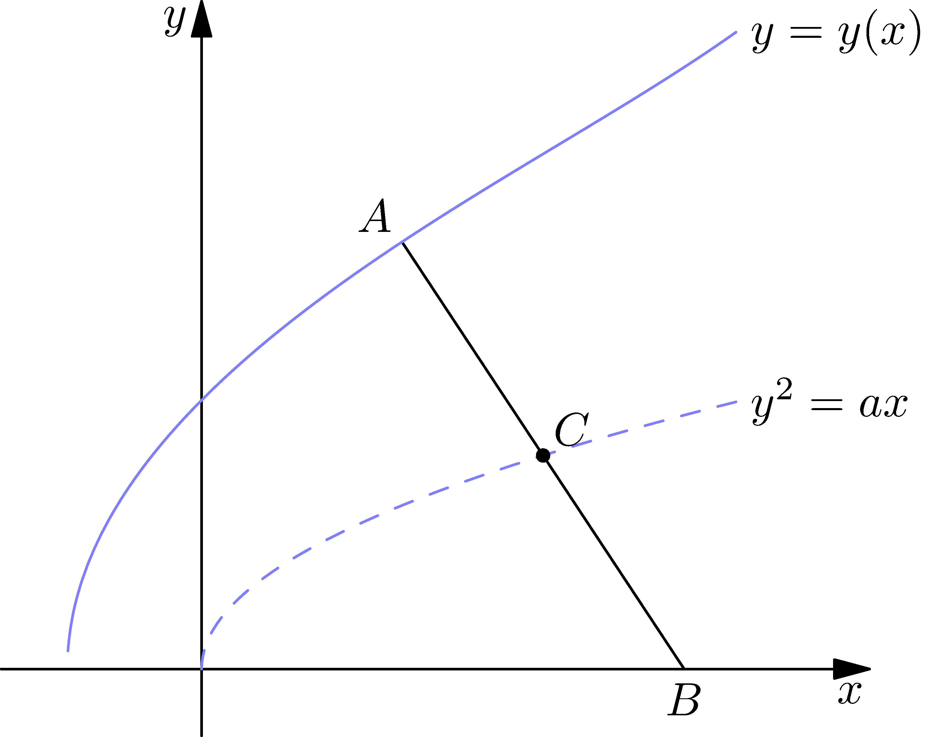
Let us consider the curve y = y(x) that goes through point (0, K), K ≠ 0, on the ordinate. Suppose that the middle point of the normal to an arbitrary point on the curve and horizontal axis (abscissa) belongs to parabola y² = 𝑎x. Find the equation of the curve.
Solution: The slope of the tangent line to the curve is its derivative, y′(x) at any point x. First, we plot the picture. Setting some parameters,
k = 3;
a = 1;
For plotting the picture, we need a solution of the given geometric problem. It will be shown shortly that the solution function y(x) is
To determine whether Line ACB is the normal line to the curve y = y(x) at point A, the slope of Line ACB is the negative reciprocal of the slope of the tangent line to the curve at point A, which is kSlope.
kSlope
0.528287
Calculate the intercept of the normal line
bIntercept = yA - kSlope xA
5.17494
Define the normal line equation. Slope is the same as kSlope
normalLine[x_] := kSlope x + bIntercept;
normalLine[x]
5.17494 - 0.528287 x
Chop[normalLine[xB]] == yB
True
The slope of the normal line is k = −1/y′(x). With this in hand, we find the equation of the normal line y = k x + b that goes through an arbitrary point A(x, y) on the curve and crosses abscissa at B(X, 0). Since X belongs to the normal line, we obtain
\[
0 = k\,X + b \qquad \Longrightarrow \qquad X = - \frac{b}{k} = b\,y' (x) .
\]
Substituting y − k x instead of b, yields
\[
X = - \frac{y-k\,x}{k} = x - \frac{y}{k} = x + y \cdot y'
\]
because k = −1/y′. The middle point C of the segment A B has coordinates (X₁, Y₁) that are mean values of corresponding coordinates A(x, y) and B(x + y·y′, 0), that is,
\[
X_1 = \frac{x + x + y\,y'}{2} = x + \frac{y}{2} \, y' \quad\mbox{and} \quad Y_1 = \frac{y}{2} .
\]
The coordinates of point C satisfy the equation of the parabola, y² = 𝑎x. Thus,
\[
Y_1^2 = \left( \frac{y}{2} \right)^2 = a\, X_1 \qquad \Longrightarrow \qquad X_1 = x + \frac{y}{2} \, y' = \frac{1}{a} \left( \frac{y}{2} \right)^2
\]
or
\[
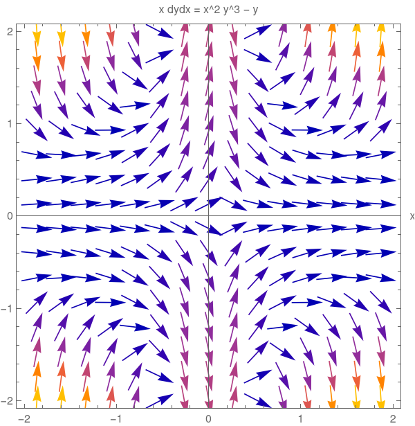
\frac{{\text d} y}{{\text d}x} = \frac{y}{2a} - \frac{2x}{y}
\tag{5.1}
\]
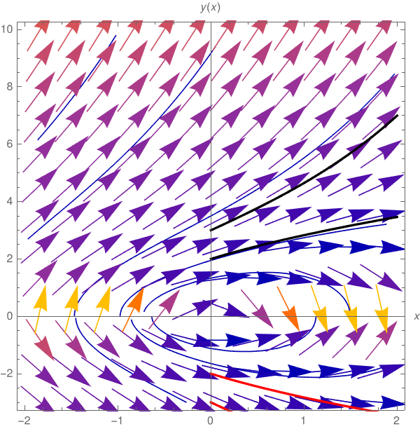
This is a Bernoulli equation. We plot the corresponding direction field and some typical solutions to Eq.(5.1).
Using the Bernoulli substitution y = u v, we obtain two separable differential equations, one for u
\[
\frac{{\text d} u}{{\text d}x} = \frac{u}{2a} \qquad \Longrightarrow \qquad u(x) = e^{x/(2a)} ,
\tag{5.2}
\]
Clear[a, u, x];
DSolve[u'[x] == u[x]/(2*a), u[x], x][[1, 1]]
{{u[x] -> E^(x/(2 a)) C[1]}}
and another one for v,
\[
u\,\frac{{\text d} v}{{\text d}x} = - \frac{2x}{u\,v} \qquad \Longrightarrow \qquad v\,\frac{{\text d} v}{{\text d}x} = - 2x\, e^{-x/a} .
\tag{5.3}
\]
Solving Eq.(5.2), we set a constant of integration to 1 because it does not matter; it is important that this constant is not zero. Integrating both sides of Eq.(5.3), we obtain
\[
\int v\,{\text d}v = \frac{v^2}{2} = - \int 2x\,e^{-x/a} \,{\text d}x = 2a \left( a+x \right) e^{-x/a} + c .
\]
{{v[x] -> -Sqrt[2] Sqrt[
2 a^2 E^(-(x/a)) + 2 a E^(-(x/a)) x + C[1]]}, {v[x] ->
Sqrt[2] Sqrt[2 a^2 E^(-(x/a)) + 2 a E^(-(x/a)) x + C[1]]}}
Integrate[-2*x*Exp[-x/a], x]
2 a E^(-(x/a)) (a + x)
We choose a constant of integration c so that v(0) = K, so
\[
\frac{1}{2}\,v(0)^2 = 2a^2 + c = K^2 /2 > 0 \qquad \Longrightarrow \qquad c = \frac{K^2}{2} -2a^2 .
\]
This leads to
\[
v^2 (x) = 4a \left( a+x \right) e^{-x/a} - 4a^2 + K^2 = 4a \left[ \left( a+x \right) e^{-x/a} - a \right] + K^2 .
\]
Taking square root, we obtain two possible formulas for function v:
\[
v(x) = \pm 2\, \sqrt{a \left( a+x \right) e^{-x/a} - a^2 + K^2 /4}
\tag{5.4}
\]
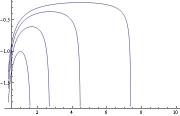
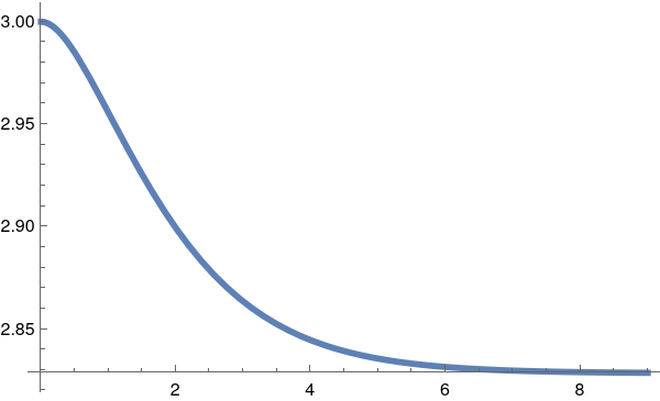
We plot one positive branch of function v(x) for K = 3.
Plot[2*Sqrt[9/4 + (a (x + a) E^(-x/a) - a^2 )] /. a -> 1, {x, 0, 9},
PlotStyle -> Thickness[0.01]]
Solution of Eq.(5,3) for K = 3.
The following animation shows the function v(x) depending on the value of K.
Now capabilities of a computer algebra systems (such as Mathematica) are so powerful that we can check equivalence of many transcendent expressions with one line command. Previously, people verified equivalence of two expressions
(one is obtained using standard command DSolve and another one was derived manually based on the Bernoulli method) were forced to evaluate these expressions at some numerical values of parameters. For example, if we were 20 years ago, we would check these two answers numerically upon evaluating the corresponding expressions at some points; for instance, we evaluate at x = 1.55.
Since these two expressions have the same numerical value, we conclude that our solution is correct and Mathematica is not ready yet to do the corresponding arithmetic manipulations.
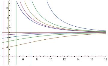
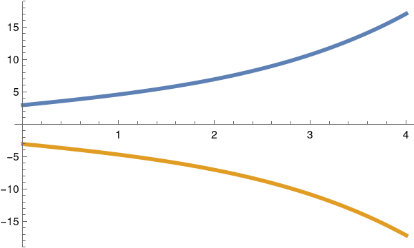
We plot both branches of the solution for two particular values of parameters: 𝑎 = 1 and K = 3.
Two branches of solution of Eq.(5,1) for 𝑎 = 1 and K = 3.
■
End of Example 5
Find the general solution of the logistic equation: y′ = y(2 - 5y).
Find a particular solution to the initial value problem: y′ = y²ex − y, y(0) = 1.
Find the general solution of the Bernoulli equation: y′ = xy³ − 3y.
Find a particular solution to the initial value problem: y′ = y²e3x + 4y, y(0) = −1.
Find the general solution of the Bernoulli equation: y′ + 2 y + 4 xy³ = 0.
For the Bernoulli equation y′ = y³ex − 2y, find the positive solution that separates solutions tending to zero from those having a vertical asymptote at a positive value of x. What is the initial value y(0) for this solution?
Azevedo, D. and Valentino, M.C., Generalization of the Bernoulli ODE, International Journal of Mathematical Education in Science and Technology, 2017, Volume 48, Issue 2, pp. 256--260; doi:https://doi.org/10.1080/0020739X.2016.1201599
Tisdell, C.C., Alternate solution to generalized Bernoulli equations via an integrating factor: an exact differential equation approach, International Journal of Mathematical Education in Science and Technology, 2017, Volume 48, Issue 6, pp. 913--918; doi: https://doi.org/10.1080/0020739X.2016.1272143
Return to Mathematica page
Return to the main page (APMA0330)
Return to the Part 1 (Plotting)
Return to the Part 2 (First Order ODEs)
Return to the Part 3 (Numerical Methods)
Return to the Part 4 (Second and Higher Order ODEs)
Return to the Part 5 (Series and Recurrences)
Return to the Part 6 (Laplace Transform)
Return to the Part 7 (Boundary Value Problems)