Return to computing page for the second course APMA0340
Return to computing page for the fourth course APMA0360
Return to Mathematica tutorial for the first course APMA0330
Return to Mathematica tutorial for the second course APMA0340
Return to Mathematica tutorial for the fourth course APMA0360
Return to the main page for the course APMA0330
Return to the main page for the course APMA0340
Return to the main page for the course APMA0360
Return to Part VI of the course APMA0330
Glossary
Preface
This section discusses a qualitative approach to the study of differential equations, and obtain qualitative information about the solutions directly from the differential equation, without actuallly finding a solution formula.
Direction Fields
For any differential equation in normal form
A striking way to visualize direction fields uses a magnet with iron filings dusted over a thin card placed horizontally and immediately above the magnet. Each iron filing becomes magnetized and tends to set itself in the direction of the resultant force at its mid-point. If the arrangement of the fillings is aided by gently tapping the card, the filings will distribute themselves approximately along the lines of force. Hence, each individual filing acts as a line-element through its mid-point. You can see many images of this at Google Images, putting "google images iron filings over a magnet" in your browser search bar.
Direction fields could be visualized by plotting a list of vectors
that are tangent to solution curves. It is as if we had a traffic policeman stationed at each point (x,y) on the plane and directed the traffic to flow along the direction specified by the slope function f(x,y). From this point of view, a solution is a curve that obeys the law at each of its points.
Correspondingly, Mathematica uses a special command to plot direction fields: VectorPlot.
It requires vector-valued input: one for abscissa (usually labeled by
x or t) and another for ordinate. Therefore, to plot a direction field for a first order differential
equation \( {\text d}y / {\text d}x = f(x,y) , \) a user needs to set 1 for the first
coordinate and f(x,y) for the second one, so making the vector input
\( \left( 1, f(x,y) \right) . \) Besides, Mathematica also offers their variations:
ListVectorPlot,
VectorDensityPlot, and
ListVectorDensityPlot.
Their applications will be clear from presented examples here and within first two parts.
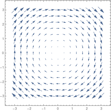
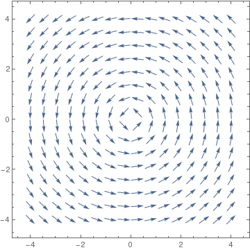
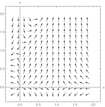
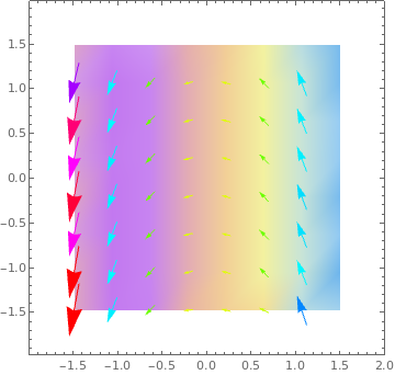
Since by default, VectorPlot automatically enlarges/stretches the lengths of vectors, Mathematica offers an option, VectorScale to suppress changes in vector lengths. Let us look at two outputs generated without and with this option:
 |
 |
pts = {{1.35386, 2.68245}, {0.416358, 1.05865}};
ptsG = Graphics[{{PointSize[Medium], Orange, Point[pts[[1]]]}, {PointSize[Medium], Blue, Point[pts[[2]]]}}];
cir = Graphics[{Circle[pts[[1]], .1], Circle[pts[[2]], .1]}];
Show[vp1, ptsG , cir]
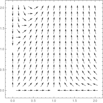
Sometimes we need to include axes into the direction field; this can be achieved, for instance, by enlarging the plotted area, as the following examples show.
vp1 = VectorPlot[ sys1 /. {a -> 1/4, b -> 2, r -> 1}, {u, 0, 2}, {v, 0, 2}, VectorScale -> {0.045, 0.9, None}, VectorStyle -> {GrayLevel[0.2]}, Axes -> True, AxesLabel -> {x, y}, AxesOrigin -> {0, 0}];
sys2 = {u (1 - u + a v), r v (1 - v + b u)};
vp2 = VectorPlot[ sys2 /. {a -> 1/4, b -> 2, r -> 1}, {u, -0.2, 2}, {v, -0.2, 2}, VectorScale -> {0.045, 0.9, None}, VectorStyle -> {GrayLevel[0.2]}, Axes -> True, AxesLabel -> {x, y}, AxesOrigin -> {0, 0}];
GraphicsRow[{vp1, vp2}, Frame -> All]
 |
 |
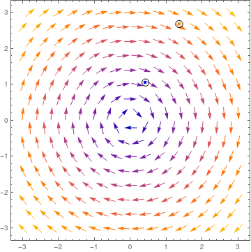
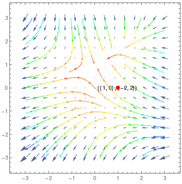
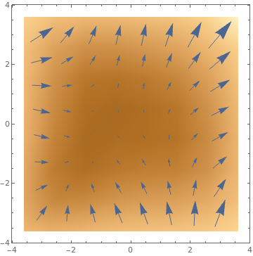
Ideally we'd get something like a tool-tip which shows the x,y position where I click (or where the mouse is currently hovering) and the evaluated vector (or scalar in the case of a scalar field) at that position. I think this would be a great way to "get a feel for" the values because by default the arrows are scaled automatically so they fit so I don't know anything about the relative magnitude of a particular arrow.
|
DynamicModule[{pt = {1, 0}},LocatorPane[Dynamic[pt],
VectorPlot[f[x, y], {x, -3, 3}, {y, -3, 3}, StreamPoints -> Coarse, StreamColorFunction -> Hue, Epilog -> Dynamic@Inset[{pt, f @@ pt}, pt], PerformanceGoal -> "Quality"], AutoAction -> True, Appearance -> Style["\[FilledCircle]", Red]]] |
 |
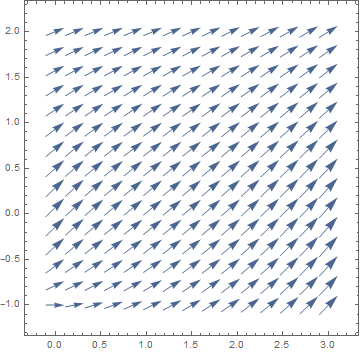
We show how to use them by examples.
|
VectorPlot[{1, (y + Exp[x/2])/(x + Exp[y])}, {x, 0, 3}, {y, -1, 2}] |
 |
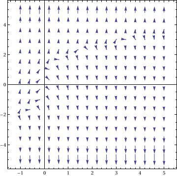
One can draw the direction field either with arrows
|
VectorPlot[{1, y^3 - 8*x}, {x, -1, 5}, {y, -5, 5}, VectorPoints -> 16, VectorStyle -> Arrowheads[0.028], Axes -> True]
|
 |
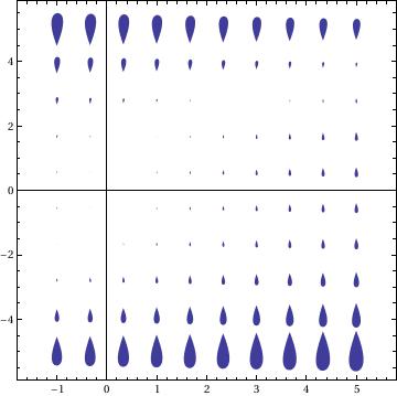
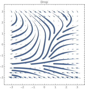
or with drop feature
|
VectorPlot[{1, y^3 - 8*x}, {x, -1, 5}, {y, -5, 5}, VectorPoints -> 10, VectorStyle -> "Drop", Axes -> True]
|
 |
|
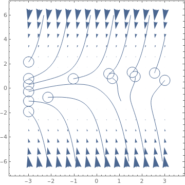
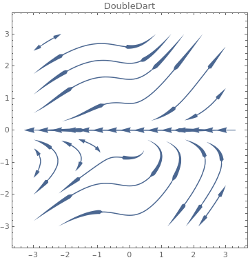
VectorPlot[{-1 - y^2 + x, 1 + x - 2 y^3}, {x, -3, 3}, {y, -6, 6},
StreamPoints -> Coarse, StreamScale -> Full,
StreamStyle -> Arrowheads[{{0.03, Automatic, Graphics[Circle[]]}}]]
|
 |
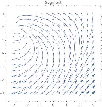
|
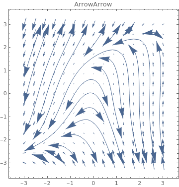
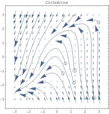
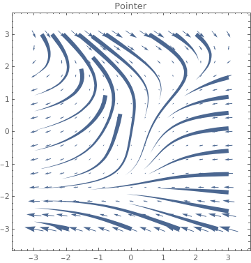
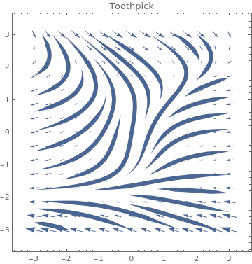
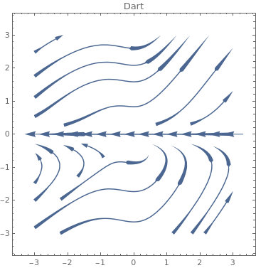
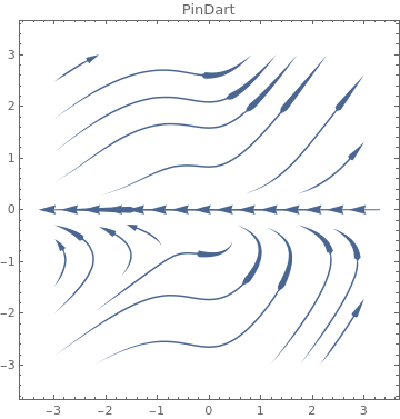
Table[VectorPlot[{-1+x^2-3y,7+2x-y},{x,-3,3},{y,-3,3},PlotLabel->s,StreamPoints->Coarse,StreamScale->{Full,All,0.05},StreamStyle->s],{s,{"Segment","Line"}}]
|
 |
 |
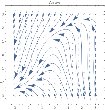
3}, PlotLabel -> s, StreamPoints -> Coarse,
StreamScale -> {Full, All, 0.05},
StreamStyle -> s], {s, {"Arrow", "ArrowArrow", "CircleArrow"}}]
 |
 |
 |
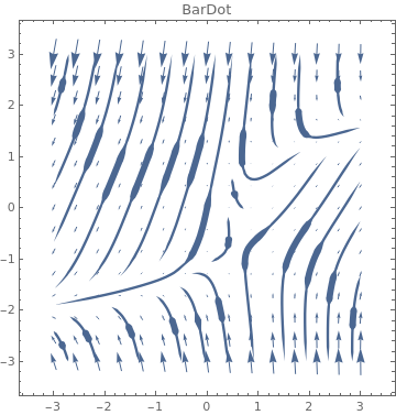
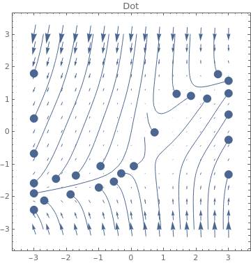
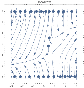
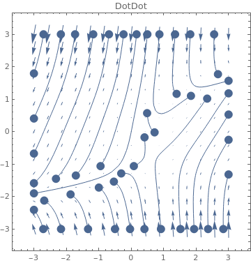
3}, {y, -3, 3}, PlotLabel -> s, StreamScale -> {Full, All, 0.03}, StreamPoints -> Coarse,
StreamStyle -> s], {s, {"BarDot", "Dot", "DotArrow", "DotDot"}}
 |
 |
 |
 |
 |
 |
 |
 |
 |
 |
 |
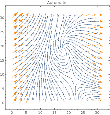
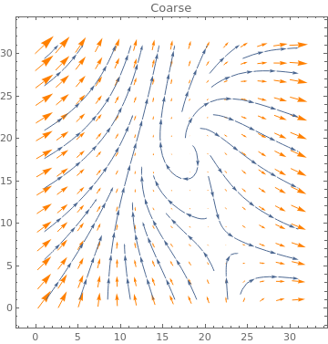
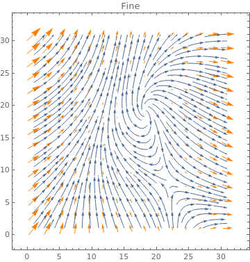
ListVectorPlot
Table[ListVectorPlot[data, VectorStyle -> Orange, StreamPoints -> p,
PlotLabel -> p], {p, {Automatic, Coarse, Fine}}]
 |
 |
 |
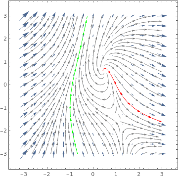
ListVectorPlot[data, DataRange -> {{-3, 3}, {-3, 3}}, StreamStyle -> Gray,
StreamPoints -> {{{{1, 0}, Red}, {{-1, -1}, Green}, Automatic}}]
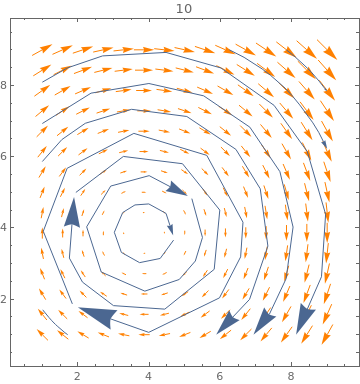
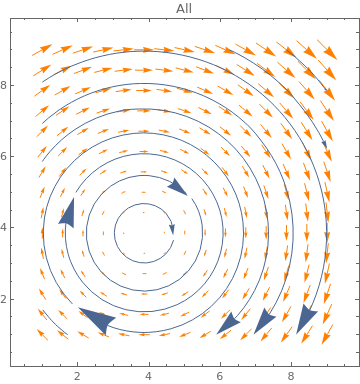
Table[ListVectorPlot[data, PlotLabel -> n, VectorStyle -> Orange,
StreamPoints -> Coarse, StreamScale -> {Full, n}], {n, {10, All}}]
 |
 |
VectorDensityPlot
VectorDensityPlot[{1, f[x, y]}, {x, 1, 4}, {y, -15, 1}, AspectRatio -> 1/GoldenRatio]
VectorDensityPlot[{-1 + x^2 + y, 1 + x + y^2}, {x, -3, 3}, {y, -3, 3}, VectorPoints -> 8]
 |
 |
 |
 |
 |
VectorDensityPlot[{-1 + 2 x^2 + y, 1 - 3 x + y^2}, {x, -3, 3}, {y, -3, 3}, VectorPoints -> 18, VectorStyle -> Arrowheads[0]]
 |
 |
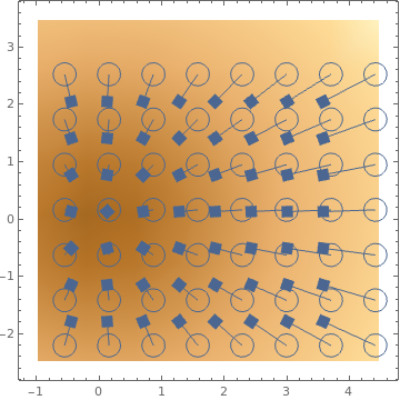
VectorStyle -> Arrowheads[{{0.03, Automatic,
Graphics[Rectangle[{-0.5, -0.5}, {0.5, 0.5}]]}, {0.03, Automatic, Graphics[Circle[]]}}]]
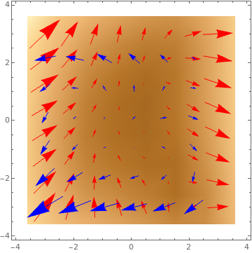
VectorDensityPlot[{{-1 + 2 x^2 + y, 1 - 3 x + y^2}, {(1 + x - y^2),
1 - .5 x^2 + y}}, {x, -3, 3}, {y, -3, 3}, VectorPoints -> 8, VectorStyle -> {Red, Blue}]
 |
 |
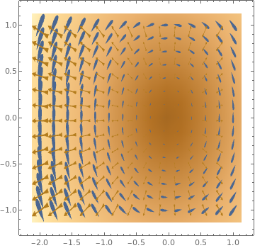
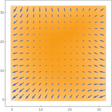
ListVectorDensityPlot
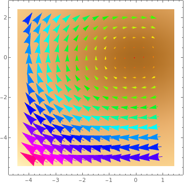
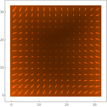
ListVectorDensityPlot[data, VectorPoints -> 8,
ColorFunction -> "Pastel", VectorColorFunction -> Hue]
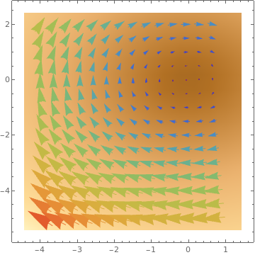
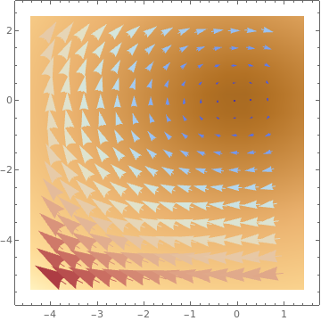
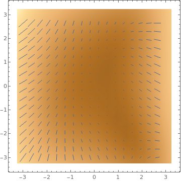
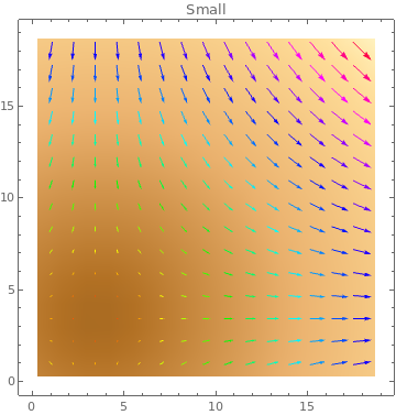
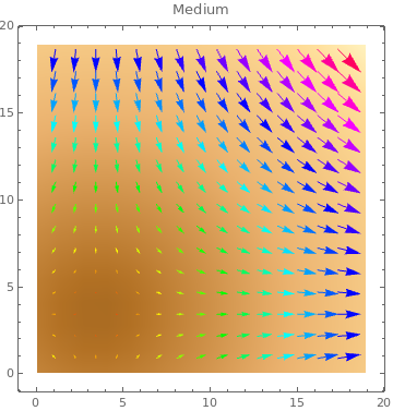
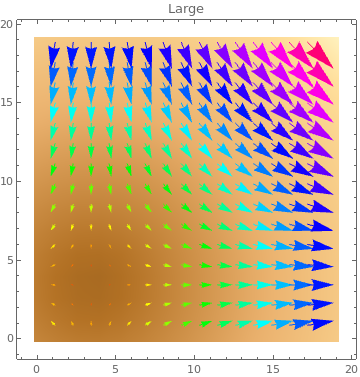
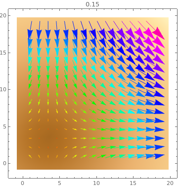
Table[ListVectorDensityPlot[data, VectorColorFunction -> Hue, PlotLabel -> s,
VectorScale -> s], {s, {Small, Medium, Large, 0.15}}]
 |
 |
 |
 |
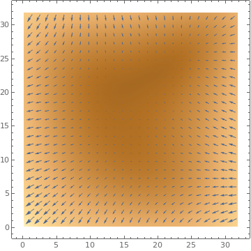
Table[ListVectorDensityPlot[data, PlotTheme -> k], {k, {"Marketing", "Detailed", "Business"}}]
 |
 |
 |
 |
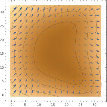
ListVectorDensityPlot[data, Mesh -> 5,
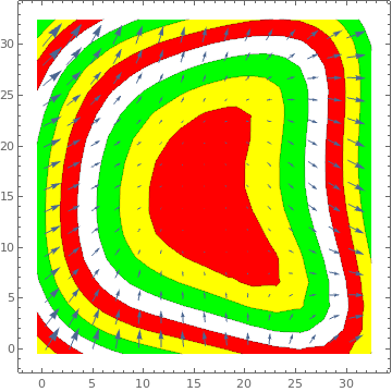
MeshFunctions -> Function[{x, y, vx, vy, n}, n]] ListVectorDensityPlot[data, Mesh -> 10,
MeshShading -> {Red, Yellow, Green, None}]
 |
 |
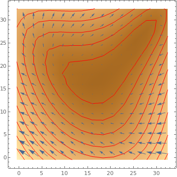
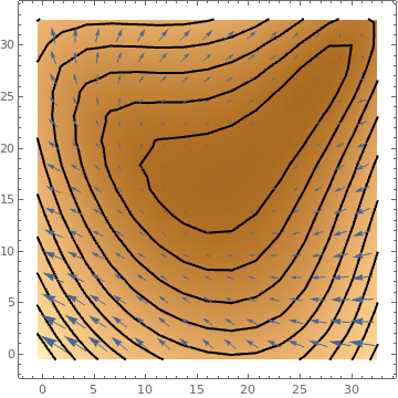
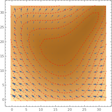
Table[ListVectorDensityPlot[data, Mesh -> 10,
MeshStyle -> s], {s, {Red, Thick, Directive[Red, Dashed]}}]
 |
 |
 |
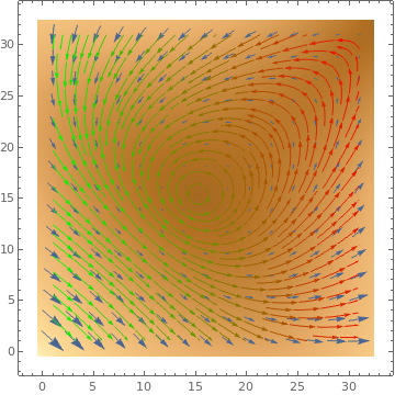
ListVectorDensityPlot[data, StreamPoints -> Fine, StreamColorFunction ->
Function[{x, y, vx, vy, n}, Blend[{Green, Red}, x]]]
Return to Mathematica page
Return to the main page (APMA0330)
Return to the Part 1 (Plotting)
Return to the Part 2 (First Order ODEs)
Return to the Part 3 (Numerical Methods)
Return to the Part 4 (Second and Higher Order ODEs)
Return to the Part 5 (Series and Recurrences)
Return to the Part 6 (Laplace Transform)
Return to the Part 7 (Boundary Value Problems)