Return to computing page for the first course APMA0330
Return to computing page for the second course APMA0340
Return to computing page for the fourth course APMA0360
Return to Mathematica tutorial for the first course APMA0330
Return to Mathematica tutorial for the second course APMA0340
Return to Mathematica tutorial for the fourth course APMA0360
Return to the main page for the course APMA0330
Return to the main page for the course APMA0340
Return to the main page for the course APMA0360
Return to Part II of the course APMA0330
To solve Clairaut's equation, one differentiates with respect to x, yielding
\[
\left[ x + f' \left( \frac{{\text d} y}{{\text d}x} \right) \right] \frac{{\text d}^2 y}{{\text d}x^2} = 0 .
\]
Hence, either \( \displaystyle
\frac{{\text d}^2 y}{{\text d}x^2} = 0
\)
or \( \displaystyle
x + f' \left( \frac{{\text d} y}{{\text d}x} \right) =0.
\)
In the former case, the first derivative must be a constant, \( c = {\text d}y/{\text d}x . \)
Substituting this into the Clairaut's equation, one obtains the family of straight line functions given by
\[
y(x) = C\,x + f\left( C \right) ,
\]
the so-called general solution of Clairaut's equation.
The latter case,
\[
x + f' \left( \frac{{\text d} y}{{\text d}x} \right) = 0
\]
defines only one solution y(x), the so-called singular solution, whose graph is the envelope of the graphs of the general solutions. The singular solution is usually represented using parametric notation, as (x(p), y(p)), where p = dy/dx.
Example 1:
With p = dy/dx, Clairaut's equation
\[
y = x\,y' + \frac{y'}{4 + (y')^2} \qquad\mbox{or} \qquad
y = x\,p + \frac{p}{4 + p^2}
\tag{1.1}
\]
has the general solution
\[
y = x\,c + \frac{c}{4 + c^2} ,
\tag{1.2}
\]
where c is an arbitrary constant.
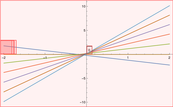
We plot a family of solutions from the general solution:
Clairaut's equations usually have singular solutions. To determine them, we rewrite the general solution in another form:
\[y \left( 4 + c^2 \right) \left( y - cx \right) = c .
-((4 + 3 c^2) x) + 2 c y = 1
\]
Upon differentiating with respect to c gives
\[
-((4 + 3 c^2) x) + 2 c y = 1 .
\]
D[(y - c*x)*(4 + c^2), c]
-((4 + 3 c^2) x) + 2 c y
This quadratic equation can be solved:
\[
c = \frac{1}{3x} \left[ y \pm \sqrt{y^2 -3x - 12 x^2} \right[ .
\tag{1.3}
\]
Solve[-((4 + 3 c^2) x) + 2 c y == 1, c]
{{c -> (y - Sqrt[-3 x - 12 x^2 + y^2])/(3 x)}, {c -> (
y + Sqrt[-3 x - 12 x^2 + y^2])/(3 x)}}
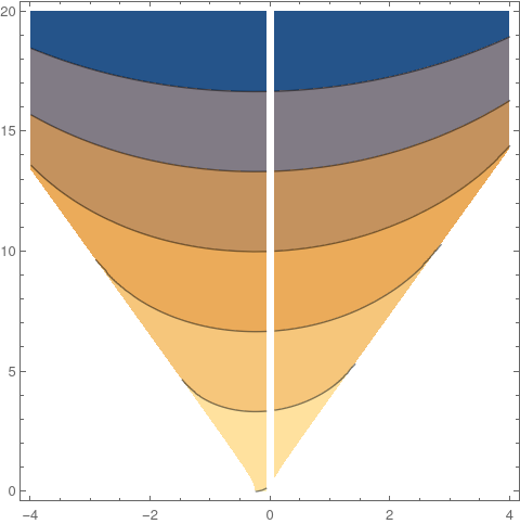
Each braanch of quadratic solution is substituting into the general solution (1.2). Mathematica helps to visialize singular solutions *the vertical line x = 0 must excluded)
c = (y - Sqrt[-3 x - 12 x^2 + y^2])/(3 x);
Simplify[c*x + c/(4 + c^2) - y]
1/3 (-2 y - Sqrt[-3 x - 12 x^2 + y^2] + (
y - Sqrt[-3 x - 12 x^2 + y^2])/(
x (4 + (y - Sqrt[-3 x - 12 x^2 + y^2])^2/(9 x^2))))
ContourPlot[ -2 y - Sqrt[-3 x - 12 x^2 + y^2] + (
y - Sqrt[-3 x - 12 x^2 + y^2])/(
x (4 + (y - Sqrt[-3 x - 12 x^2 + y^2])^2/(9 x^2))), {x, -4, 4}, {y,
0, 20}]
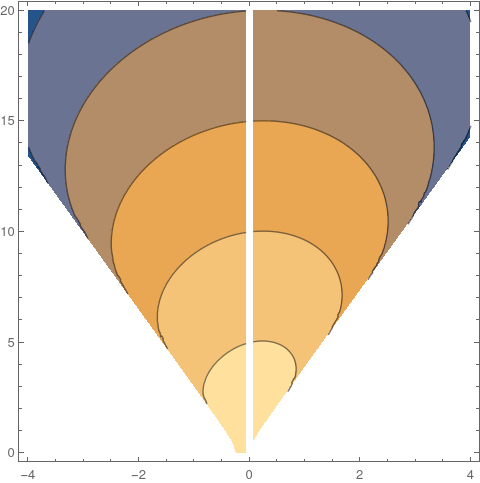
and for another branch:
c = (y + Sqrt[-3 x - 12 x^2 + y^2])/(3 x);
Simplify[c*x + c/(4 + c^2)-y]
1/3 (-2 y + Sqrt[-3 x - 12 x^2 + y^2] + (
y + Sqrt[-3 x - 12 x^2 + y^2])/(
x (4 + (y + Sqrt[-3 x - 12 x^2 + y^2])^2/(9 x^2))))
ContourPlot[-2 y + Sqrt[-3 x - 12 x^2 + y^2] + (
y + Sqrt[-3 x - 12 x^2 + y^2])/(
x (4 + (y + Sqrt[-3 x - 12 x^2 + y^2])^2/(9 x^2))), {x, -4, 4}, {y,
0, 20}]
Implicit plot for negative branch.
Implicit plot for positive branch.
■
Example 2:
We consider another Clairaut's equation
If we return to the case when y'' = 0, then we have a linear solution
y = Ax + B, for some constants A and B.
If we substitute this into Clairaut’s equation, it gives
\[
A\,x + B = x\,A + A^2 \qquad \Longrightarrow \qquad B = A^2 ,
\]
and we obtain a family of solutions (called the general solution):
\[
y = x\,A + A^2 .
\]
It has the envelope (singular solution) \( \displaystyle y = - \frac{x^2}{4} . \)
If we substitute \( \displaystyle y = z - \frac{x^2}{4} \) into Clairaut's equation, we obtain a differential equation
Solving the differential equation for z, we get its general solution depending on two arbitrary constants:
\[
z(x) = \begin{cases} \frac{1}{4} \left( x- a \right)^2 , & \ x \leqslant a,
\\
0 , & \ a \leqslant x \leqslant b ,
\\
\frac{1}{4} \left( x- b \right)^2 , & \ x \geqslant b,
\end{cases}
\]
where 𝑎 and b are constants satisfying -∞ ≤ 𝑎 ≤ b ≤ ∞.
■
Generalized Clairaut's equation
The differential equation
\[
f \left( x\,\frac{{\text d} y}{{\text d}x}-y \right) = g \left( \frac{{\text d} y}{{\text d}x} \right) ,
\]
where f and g are some given smooth functions, can be solved in exactly the same manner as Clairaut's equation to obtain the general solution
\[
f \left( x\,C-y \right) = g \left( C \right) ,
\]
where C is an arbitrary constant. The generalized Clairaut's equation may also have a singular solution. If it does, it can be obtained by
differentiating the above equation with respect to x to obtain
\begin{equation}
y''\left[ f'(xy'-y)x-g'(y') \right] =0.
\label{clair:c}
\end{equation}
If the first term in the above equation is zero, then
the generalized Clairaut's equation is recovered. If the second term in
the equation is zero, then two equations
can be solved together to
eliminate y'. The resulting equation for y=y(x) will have no arbitrary constants and so will be a singular solution.
Example 3:
Consider the generalized Clairaut's equation
\[
(xy'-y)^2-(y')^2-1=0.
\]
Since this is a generalized Clairaut's equation with f(p) = p² and g(p) = p² -1, its general solution becomes
To find the singular solution, we differentiate the given equation with respect to x to obtain
\begin{equation}
y''[2(xy'-2)x-2y']=0.
\end{equation}
If the second term is set equal to zero, then we find
\begin{equation}
y'=\frac{x y}{x^2-1}.
\label{clair:g}
\end{equation}
We determine the
singular solution to be
%
\begin{equation}
x^2+y^2=1.
\label{clair:h}
\end{equation}
Note that this equation is not derivable from the general solution
for any choice of C.
■
The Lagrange differential equation
A differential equation of type
\[
y = x\, f(y' ) + g(y' ) ,
\]
where f and g are given functions differentiable on a certain interval, is called the Lagrange equation. It is convenient to denote by p = dy/dx, the derivative of the unknown function. Then differentiating the equation \( \displaystyle y = x\,f(p) + g(p), we obtain
This is a first-order differential equation, and its solution x(p) should be achievable
depending on the details of the functions f(p) and g(p). Even its singular solution
may be found be setting the singular value p = f(p) in the original differential equation.
Example 4:
Consider the differential equation
\[
y = 3p\,x + 7\,\ln p, \qquad p = {\text d}y/{\text d}x .
\]
The last two equations provide the parametric representation of the general solution y = y(x). A singular solution is y(x) = 0.
■
Return to Mathematica page
Return to the main page (APMA0330)
Return to the Part 1 (Plotting)
Return to the Part 2 (First Order ODEs)
Return to the Part 3 (Numerical Methods)
Return to the Part 4 (Second and Higher Order ODEs)
Return to the Part 5 (Series and Recurrences)
Return to the Part 6 (Laplace Transform)
Return to the Part 7 (Boundary Value Problems)