Preface


This section treats constant coefficient linear differential equations. It serves as a clarification of the previous section in case of constant coefficients differential operators.

Return to computing page for the first course APMA0330
Return to computing page for the second course APMA0340
Return to Mathematica tutorial for the first course APMA0330
Return to Mathematica tutorial for the second course APMA0340
Return to the main page for the course APMA0330
Return to the main page for the course APMA0340
Return to Part IV of the course APMA0330

Constant Coefficient ODEs


Linear constant coefficient differential equations form an important class of differential equations that appear both in physical models and as approximations for more complicated equations. For example, the second part of this tutorial uses the solving methods of constant coefficient equations to extend them to systems of differential equations. We start with second order equations because all steps become transparent and can be performed by utilizing solution solvers.


Second order equations with constant coefficients


We consider the second order homogeneous constant coefficient differential equation
\begin{equation} \label{EqConstant.1} a\,y'' + b\,y' + c\,y = 0, \end{equation}
where the coefficients 𝑎 ≠ 0, b, and c are real constants and prime indicates the derivative with respect to independent variable \( y' = \texttt{D} \,y = {\text d}y/{\text d}x \) and \( y'' = \texttt{D}^2 y = {\text d}^2 y/{\text d}x^2 . \) From the section on linear Ordinary Differential Equations we know that the general solution of Eq.\eqref{EqConstant.1} will be of the form
\begin{equation} \label{EqConstant.2} y(x) = c_1 y_1 (x) + c_2 y_2 (x) , \end{equation}
where { y1, y2 } is a fundamental set of solutions for the given differential equation \eqref{EqConstant.1}. It is not hard to verify that the second order linear constant coefficient differential equation \eqref{EqConstant.1} has at least one solution of the form \( y = e^{\lambda x} . \) Substituting the exponential function into the differential equation gives
\[ a \left( e^{\lambda x} \right)'' + b \left( e^{\lambda x} \right)' + c \left( e^{\lambda x} \right) = 0 \qquad\mbox{or} \qquad a\,\lambda^2 e^{\lambda x} + b\,\lambda e^{\lambda x} + c\, e^{\lambda x} = 0 . \]
Finally, dividing by \( e^{\lambda x} \ne 0 , \) we get
\begin{equation} \label{EqConstant.3} a\,\lambda^2 + b\,\lambda + c = 0 . \end{equation}
This polynomial is called the characteristic polynomial of the differential equation \( a\,y'' + b\,y' + c\,y = 0 . \) It is easy to identify the characteristic equation when the corresponding differential equation is written in operator form:
\[ L \left[ \texttt{D} \right] y = \left( a\,\texttt{D}^2 + b\,\texttt{D} + c\,\texttt{I} \right) y = 0 , \]
where \( \texttt{D} = {\text d}/{\text d}x \) is the derivative operator (in Euler's notation) and D0 = I is the identity operator. Then just substituting λ instead of D leads to the characteristic polynomial. We summarize the construction of the fundamental set of solution to constant coefficient homogeneous differential equations of the second order in the following statement.

Procedure for solution of second order differential equation with constant coefficients: To solve the second order constant coefficient differential equation \( a\,y'' + b\,y' + c\,y = 0 \) follow the following steps.

  1. Form the characteristic equation \( a\,\lambda^2 + b\,\lambda + c = 0 \) and determine its roots and their multiplicities.
  2. The corresponding a fundamental set of solutions is determined as follows.
  3. If λ1 and λ2 are two unequal real roots of the characteristic equation (when b² > 4𝑎c), the general solution is
    \[ y = c_1 e^{\lambda_1 x} + c_2 e^{\lambda_2 x} , \]
    with some arbitrary constants c1 and c2.
  4. If λ is a real root of multiplicity 2 (when b² = 4𝑎c), then \( y_1 = e^{\lambda x} , \ y_2 = x\, e^{\lambda x} \) form a fundamental set of solutions, so the general solution becomes \( y = c_1 \, e^{\lambda x} + c_2 x\, e^{\lambda x} . \)
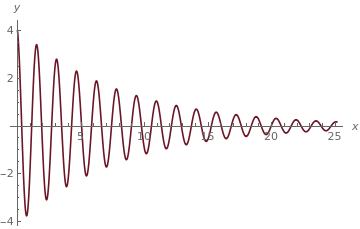
  5. If λ1, λ2 are complex roots (when b² < 4𝑎c), then they are a complex conjugate pair \( \lambda_1 = \alpha + {\bf j} \beta , \quad \lambda_2 = \alpha - {\bf j} \beta , \) where j is the unit vector in positive vertical direction on the complex plane ℂ so j² = -1. The general solution is
    \[ y = c_1 e^{\alpha x} \,\cos (\beta x) + c_2 e^{\alpha x} \,\sin (\beta x) = e^{\alpha x} \left( c_1 \cos (\beta x) + c_2 \sin (\beta x) \right) . \]

Example: Consider the linear differential equation

\[ y'' + y' -6\,y = 0 , \]
to which corresponds the linear differential operator L[D] = (D - 2)(D + 3). The characteristic polynomial has two distinct real roots
\[ L \left( \lambda \right) = (\lambda -2)(\lambda +3) . \]
Therefore, the general solution of the differential equation is
\[ y (x) = c_1 e^{-3x} + c_2 e^{2x} . \]
Their Wronskian is
\[ W\left[ e^{-3x} ,e^{2x} \right] = \det \begin{bmatrix} e^{-3x} & e^{2x} \\ -3\,e^{-3x} & 2\,e^{2x} \end{bmatrix} = 5\,e^{-x} \ne 0. \]
   ■

Example: Consider the linear differential equation

\[ y'' - 4\,y' +4\,y = 0 , \]
to which corresponds the linear differential operator L[D] = (D - 2)². The characteristic polynomial has one double real root
\[ L \left( \lambda \right) = (\lambda -2)^2 . \]
Therefore, the general solution of the above differential equation is
\[ y = c_1 e^{2x} + c_2 x\,e^{2x} . \]
We check with Mathematica:
Factor[k^2 -4*k + 4]
Solve[k^2 -4*k + 4 == 0]
DSolve[y''[x] -4*y'[x] +4*y[x] == 0, y[x],x]
   ■

Example: Consider the differential equation

\[ 16\,y'' +8\,y' +145\,y = 0 , \]
to which corresponds the linear differential operator L[D] = 16 D² + 8 D + 145. The characteristic polynomial
\[ L \left( \lambda \right) = 16 \left[ \left( \lambda + \frac{1}{4} \right)^2 +9 \right] \]
has a pair of complex conjugate roots. Therefore, the general solution of the above differential equation is
\[ y = c_1 e^{-x/4} \cos (3x) + c_2 \,e^{-x/4} \sin (3x) . \]
Factor[16*k^2 + 8*k + 145, GaussianIntegers -> True]
Solve[[16*k^2 + 8*k + 145 == 0]
DSolve[16*y''[x] + 8*y'[x] + 145*y[x] == 0, y[x],x]
   ■

Example: Consider the initial value problem

\[ 64\,y'' +16\,y' +1025\,y = 0 , \qquad y(0) = 4, \quad y' (0) = -9/2 . \]
First, we find the general solution
gensol = Simplify[ DSolve[64*y''[x] + 16*y'[x] + 1025*y[x] == 0, y[x], x]] // Flatten
E^(-x/8) (C[2] Cos[4 x] + C[1] Sin[4 x])}
\[ y = e^{-x/8} \left( C_1 \cos 4x + C_2 \sin 4x \right) . \]
Next, we find two linearly independent solutions from two initial value problems:
\begin{align*} 64\,y'' + 16\,y' + 1025\, y &= 0, \qquad y(0) =1, \quad y'(0) =0; \\ 64\,y'' + 16\,y' + 1025\, y &= 0, \qquad y(0) =0, \quad y'(0) =1. \end{align*}
sol1 = DSolve[{64*y''[x] + 16*y'[x] + 1025*y[x] == 0, y[0] == 1, y'[0] == 0}, y[x], x]// Flatten
{y[x] -> 1/32 E^(-x/8) (32 Cos[4 x] + Sin[4 x])}
sol2 = DSolve[{64*y''[x] + 16*y'[x] + 1025*y[x] == 0, y[0] == 0, y'[0] == 1}, y[x], x]// Flatten
{y[x] -> 1/4 E^(-x/8) Sin[4 x]}
Therefore, we have
\[ y_1 = e^{-x/8} \left( \cos (4x) + \frac{1}{32} \,\sin (4x) \right) , \qquad y_2 = \frac{1}{4}\, e^{-x/8} \sin (4x) . \]
We can also determine these functions from the general solution.
e1 = y[x] /. gensol[[1]] /. x -> 0
C[2]
Computing the derivative
e2 = D[y[x] /. gensol[[1]], x] /. x -> 0
4 C[1] - C[2]/8
Solving for c1 and c2 shows that
Solve[{C[2] == 1, 4 C[1] - C[2]/8 == 0}, {C[2], C[1]}]
{{C[2] -> 1, C[1] -> 1/32}}
So \( c_1 = 1/32, \ c_2 = 1 , \) and we get
\[ y_1 = e^{-x/8} \left( \cos (4x) + \frac{1}{32} \,\sin (4x) \right) . \]
Similarly, we can construct \( y_2 (x) = \frac{1}{4}\, e^{-x/8} \sin 4x . \) Then the required solution of the initial value problem will be
\[ y = 4\, y_1 (x) - \frac{9}{2}\,y_2 (x) = e^{-x/8} \left[ 4\,\cos (4x) - \sin (4x) \right] . \]
Finally, we plot the solution:
Plot[E^(-x/8) (4 Cos[4 x] - Sin[4 x]), {x, 0, 8*Pi}, AxesLabel -> {x, y}, PlotStyle -> CMYKColor[0, 0.79, 0.64, 0.58]]
      The solution to the initial value problem.
   ■


Linear homogeneous constant coefficient equations of arbitrary order


Consider linear differential equation with constant coefficients
\begin{equation} \label{EqConstant.4} a_n \, y^{(n)} + a_{n-1} \, y^{(n-1)} + \cdots + a_1 \, y' + a_0 \, y= 0 , \end{equation}
where all coefficients \( a_0, a_1 , \ldots , a_n \ne 0 \) are constants. It is convenient to associate with the left-hand side a linear differential operator
\begin{equation} \label{EqConstant.5} L \left[ \texttt{D} \right] = a_n \,\texttt{D}^n + a_{n-1} \, \texttt{D}^{n-1} + \cdots + a_1 \, \texttt{D} + a_0 \,\texttt{I} , \end{equation}
where \( \texttt{D} = {\text d} / {\text d}x \) is the derivative operator (with respect to independent variable x), and D0 = I is the identical operator. Following L. Euler, we substitute into the homogeneous linear differential equation L[D] y = 0 the exponential function \( y(x) = e^{\lambda x} , \) to obtain
\] a_n \,\lambda^n e^{\lambda x} + a_{n-1} \,\lambda^{n-1} e^{\lambda x} + \cdots + a_1 \,\lambda \,e^{\lambda x} + a_0 e^{\lambda x} = 0 \]
because of the well-known derivative rule: \( \texttt{D} \,e^{\lambda x} = \lambda \,e^{\lambda x} . \) Factoring the exponential term out because \(e^{\lambda x} \ne 0 , \) we get the polynomial equation
\begin{equation} \label{EqConstant.6} a_n \,\lambda^n + a_{n-1} \,\lambda^{n-1} + \cdots + a_1 \,\lambda + a_0 = 0 , \end{equation}
which deserve a special name.
Definition: For every linear differential operator with constant coefficients \( L \left[ \texttt{D} \right] = a_n \,\texttt{D}^n + a_{n-1} \, \texttt{D}^{n-1} + \cdots + a_1 \, \texttt{D} + a_0 \,\texttt{I} , \) corresponds a polynomial
\[ L\left( \lambda \right) = a_n \,\lambda^n + a_{n-1} \,\lambda^{n-1} + \cdots + a_1 \,\lambda + a_0 , \]
which is called the characteristic polynomial for the linear operator L[D] or differential equation \( L\left[ \texttt{D} \right] y = 0 . \) Equating the characteristic polynomial to zero, we obtain the characteristic equation: L(λ) = 0.
If we factor the characteristic polynomial into a product of simple terms (according to the fundamental theorem of algebra) , we obtain
\begin{equation} \label{EqConstant.7} L\left( \lambda \right) = a_n \left( \lambda - k_1 \right)^{m_1} \left( \lambda - k_2 \right)^{m_2} \cdots \left( \lambda - k_r \right)^{m_r} . \end{equation}
Here k1, k2, … , kr are distinct roots (or nulls) of the polynomial equation L(λ) = 0, and m1, m2, … ,mr are multiplicities of the roots. If m = 1, the corresponding root is called simple. To each root k of multiplicity m corresponds a set of m linearly independent functions
\[ \left\{ e^{k\,x} , x\,e^{k\,x} , \ldots , x^{m-1} e^{k\,x} \right\} , \]
of total m1 + m2 + ··· + mr = n, the order of the characteristic polynomial, which is the same as the order of the differential operator L[D].

Therefore, if all roots of the characteristic equation L(λ) = 0 are distinct and real, then the general solution of linear constant coefficient differential equation L[D] y = 0 is

\begin{equation} \label{EqConstant.8} y(x) = c_1 e^{k_1 x} + c_2 e^{k_2 x} + \cdots + c_n e^{k_n x} , \end{equation}
where c1, c2, … ,cn are arbitrary constants. Hence, the problem of solving constant coefficient linear differential equation is reduced to an algebra problem for finding roots of characteristic equation and determination of their multiplicities. We consider in next two sections the cases when roots are complex numbers or are of multiplicity greater than 1.

Procedure for solution of arbitrary order differential equation with constant coefficients: To solve the n-th order constant coefficient differential equation \( a_n \, y^{(n)} + a_{n-1} \, y^{(n-1)} + \cdots + a_1 \, y' + a_0 \, y = 0 , \) follow the following steps.

  1. Form the characteristic equation \( a_n \, \lambda^n + a_{n-1} \, \lambda^{n-1} + \cdots + a_1 \, \lambda + a_0 = 0 , \) and determine its roots and their multiplicities.
  2. The corresponding a fundamental set of solutions is determined as follows.
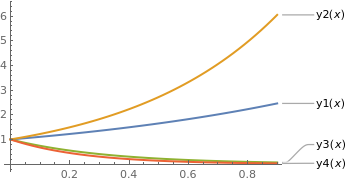
  3. If λ is a real root of multiplicity m, then include the m functions
    \[ \left\{ e^{\lambda x} , \ x\, e^{\lambda x} , \ldots , x^{m-1} e^{\lambda x} , \right\} \]
    in the fundamental set of solutions.
  4. If α ±jβ is a pair of complex conjugate roots and they each have multiplicity m, then include the 2m functions
    \[ \left\{ e^{\alpha x} \cos \beta x , \ x\, e^{\alpha x} \cos \beta x , \ldots , \ x^{m-1} e^{\lambda x} \cos \beta x , \ , e^{\alpha x} \sin \beta x , \ x\, e^{\alpha x} \sin \beta x , \ldots , \ x^{m-1} e^{\lambda x} \sin \beta x \right\} \]
    in the fundamental set of solutions.
Recall that a polynomial L(λ) has a root (or null) of multiplicity m if it can be factored as L(λ) = (λ - r)^m p(λ), where the polynomial p(λ) is not zero at λ = r: p(r) ≠ 0.

Example: Consider the linear differential equation

\[ y''' - y'' -8\,y' +12\,y = 0 , \]
to which corresponds the linear differential operator L[D] = (D - 2)²(D + 3). The characteristic polynomial has two distinct real roots
\[ L \left( \lambda \right) = (\lambda -2)^2 (\lambda +3) . \]
Therefore, the general solution of the above differential equation is
\[ y (x) = c_1 e^{-3x} + c_2 e^{2x} + c_3 x\,e^{2x} . \]
Their Wronskian is
Simplify[Wronskian[{Exp[-3*x], Exp[2 x], x*Exp[2*x]}, x]]
\[ W\left[ e^{-3x} ,e^{2x} , x\,e^{2x} \right] = \det \begin{bmatrix} e^{-3x} & e^{2x} & x\,e^{2x} \\ -3\,e^{-3x} & 2\,e^{2x} & \left( 1 + 2x \right) e^{2x} \\ 9\,e^{-3x} & 4\,e^{2x} & 4\left( 1 + x \right) e^{2x} \end{bmatrix} = 25\,e^{x} \ne 0. \]
   ■

Example: Consider the linear differential equation

\[ y^{(4)} + 4\,y^{(3)} -7\,y'' -22\,y' y' + 24\,y = 0 , \]
to which corresponds the linear differential operator L[D] = (D - 2)(D + 3) (D - 1)(D + 4). The characteristic polynomial has four distinct real roots
\[ L \left( \lambda \right) = (\lambda -2)(\lambda +3) (\lambda -1)(\lambda +4) . \]
Therefore, the general solution of the above differential equation is
\[ y (x) = c_1 e^{-3x} + c_2 e^{2x} + c_3 e^{x} + c_4 e^{-4x} . \]
Their Wronskian is
\[ W\left[ e^{-3x} ,e^{2x} , e^{x} ,e^{-4x} \right] = \det \begin{bmatrix} e^{-3x} & e^{2x} & e^{x} & e^{-4x} \\ -3\,e^{-3x} & 2\,e^{2x} & e^{x} & -4\,e^{-4x} \\ 9\,e^{-3x} & 4\,e^{2x} & e^{x} & 16\,e^{-4x} \\ -27\,e^{-3x} & 8\,e^{2x} & e^{x} & 64\,e^{-4x} \end{bmatrix} = 600\,e^{-x4} \ne 0. \]
We check with Mathematica:
Simplify[Wronskian[{Exp[-3*x], Exp[2*x], Exp[x], Exp[-4*x]}, x]]
600 E^(-4 x)
Suppose that we want to construct four linearly independent solutions to the given fourth order linear differential equation L[D] y = (D - 2)(D + 3) (D - 1)(D + 4) y = 0 by solving the corresponding initial value problems:
\begin{align*} A: & \quad y^{(4)} + 4\,y^{(3)} -7\,y'' -22\,y' y' + 24\,y = 0 , \qquad y(0) =1, \ y'(0) =0, \ y'' (0) =0, \ y'''(0) =0; \\ B: & \quad y^{(4)} + 4\,y^{(3)} -7\,y'' -22\,y' y' + 24\,y = 0 , \qquad y(0) =0, \ y'(0) =1, \ y'' (0) =0, \ y'''(0) =0; \\ C: & \quad y^{(4)} + 4\,y^{(3)} -7\,y'' -22\,y' y' + 24\,y = 0 , \qquad y(0) =0, \ y'(0) =0, \ y'' (0) =1, \ y'''(0) =0; \\ D: & \quad y^{(4)} + 4\,y^{(3)} -7\,y'' -22\,y' y' + 24\,y = 0 , \qquad y(0) =0, \ y'(0) =0, \ y'' (0) =0, \ y'''(0) =1. \end{align*}
We ask Mathematica for help to obtain the following set of linearly independent functions:
\begin{align*} y_A &= \frac{1}{5}\, e^{-4x} \left( -1 +2\,e^x +6\,e^{5x} -2\,e^{6x} \right) ; \\ y_B &= \frac{1}{30}\, e^{-4x} \left( 7 -15\,e^x + 3\,e^{5x} + 5\,e^{6x} \right) > 1; \\ y_C &= \frac{1}{20}\, e^{-3x} \left( 1 -5\,e^{4x} +4\,e^{5x} \right) > 0; \\ y_D &= \frac{1}{60}\, e^{-4x} \left( -2 +3\, e^x -3\,e^{5x} +2\,e^{6x} \right) > 0. \end{align*}
eq := D[y[x], {x, 4}] + 4*D[y[x], {x, 3}] - 7*y''[x] - 22*y'[x] + 24*y[x]
DSolve[{eq == 0, y[0] == 0, y'[0] == 0, y''[0] == 0, y'''[0] == 1}, y[x], x]
yD[x_] = 1/60 E^(-4 x) (-2 + 3 E^x - 3 E^(5 x) + 2 E^(6 x))]
yC[x_] = 1/20 E^(-3 x) (1 - 5 E^(4 x) + 4 E^(5 x))]
yB[x_] = 1/30 E^(-4 x) (7 - 15 E^x + 3 E^(5 x) + 5 E^(6 x))]
yA[x_] = 1/5 E^(-4 x) (-1 + 2 E^x + 6 E^(5 x) - 2 E^(6 x))
Their Wronskian is
Simplify[Wronskian[{yA[x], yB[x], yC[x], yD[x]}, x]]
E^(-4 x)
\[ W\left[ y_A (x) , y_B (x) , y_C (x) , y_D (x) \right] = e^{-4x} > 0. \]
We plot two sets of our four solutions:
Plot[{yA[x], yB[x], yC[x], yD[x]}, {x, 0, 1.7}, PlotStyle -> Thick, PlotLabels -> Automatic]
y1[x_] = Exp[x]; y2[x_] = Exp[2*x]; y3[x_] = Exp[-3*x]; y4[x_] = Exp[-4*x];
Plot[{y1[x], y2[x], y3[x], y4[x]}, {x, 0, 0.9}, PlotStyle -> Thick, PlotLabels -> Automatic]
    Family of linearly independent solutions.
      Family of solution from the IVPs.
   ■

Example: Consider the linear differential equation

\[ y^{(5)} +5\, y^{(4)} + 18\,y^{(3)} +34,y'' + 45\,y' y' + 25\,y = 0 , \]
to which corresponds the linear differential operator L[D] = D5 + 5 D4 + 18 D³ + 34 D² + 45 D + 25. The characteristic polynomial has two complex conjugate roots of multiplicity 2 and one simple root:
\[ L \left( \lambda \right) = \left[ (\lambda +1)^2 + 4 \right]^2 (\lambda +1) . \]
Therefore, the general solution of the above differential equation is
\[ y (x) = e^{-x} \left[ c_1 \cos 2x + c_2 x\,\cos 2x + c_3 \sin 2x + c_4 x\,\sin 2x + c_5 \right] . \]
Their Wronskian is
Simplify[Wronskian[{Exp[-x], Exp[-x]*Cos[2*x], x*Exp[-x]*Cos[2*x], Exp[-x]*Sin[2*x], x*Exp[-x]*Sin[2*x]}, x]]
\[ W \left[ e^{-x}, e^{-x} \cos 2x, x\,e^{-x} \cos 2x , e^{-x} \sin 2x , x\, e^{-x} \sin 2x \right] = 1024\, e^{-5x} \ne 0 . \]
   ■


Return to Mathematica page
Return to the main page (APMA0330)
Return to the Part 1 (Plotting)
Return to the Part 2 (First Order ODEs)
Return to the Part 3 (Numerical Methods)
Return to the Part 4 (Second and Higher Order ODEs)
Return to the Part 5 (Series and Recurrences)
Return to the Part 6 (Laplace Transform)
Return to the Part 7 (Boundary Value Problems)