A Padé approximant is the "best" approximation of a function by a rational function of given order -- under this technique, the approximant's power series agrees with the power series of the function it is approximating. The technique was developed around 1890 by the French mathematician Henri Padé (1863--1953), but goes back to the German mathematician Georg Frobenius (1849--1917) who introduced the idea and investigated the features of rational approximations of power series. Henri Eugène Padé, while preparing his doctorate under Charles Hermite, he introduced what is now known as the Padé approximant---a rational functions that provides a smallest overall error on the interval [𝑎, b].

Actually, the first rational approximation was obtained in seventh century by the Indian mathematician Bhaskara (c.600 – c.680). He has given the rule for a remarkable approximation of the sine function:

When the power series representation of a function diverges, it indicates the inability of the power series to approximate the function in a certain region. A theorem from complex analysis states that if the Taylor series of a function diverges, then that function has singularities in the complex plane. A Padé approximant is a ratio of polynomials that contains the same information that a truncated power series does. Because the polynomial in the denominator may have roots in the region of interest, the Padé approximant may accurately indicate the presence of singularities.

Given a function f and two integers \( m \ge 0 \quad\mbox{and}\quad n \ge 1, \) the Padé approximant of order [m/n] is the quotient of two polynomials P_m(x) and Q_n(x) of degrees m and n, respectively:

), is unique for given m and n, that is, the coefficients \( a_0 , \ldots , a_m , b_1 , \ldots b_n \) can be uniquely determined. There is nothing special with the chosen point x = 0. A change of variable can be used to shift the calculations over to an interval that contains zero. Example: Padé approximation of the cosine function

Example: Consider Padé approximants for cosine functions

\begin{align*} r_2 (x) &= \dfrac{1 - \frac{5}{12}\, x^2}{1 + \frac{1}{12}\, x^2} , \\ r_4 (x) &= \dfrac{1 - \frac{115}{252}\,x^2 + \frac{313}{15120}\,x^4}{1+ \frac{11}{252}\,x^2 + \frac{13}{15120}\,x^4} , \\ r_8 (x) &= \dfrac{1-\frac{260735}{545628}\,x^2 + \frac{4375409}{141863280}\,x^4 - \frac{7696415}{13108167072}\,x^6 + \frac{80737373}{23594700729600}\, x^8}{1 + \frac{12079}{545628}\, x^2 + \frac{34709}{141863280}\,x^4 + \frac{109247}{65540835360}\, x^6 + \frac{11321}{1814976979200}\, x^8} . \end{align*}

   ■

Example: Padé approximation of the solution to the autonomous equation

Example: Suppose we wish to approximate the solution of the ordinary differential equation

\[ y'=y^2,\qquad y(0)=1. \]

Since the equation is separable its solution is y(x) = 1/(1-x). If we tried to find the Taylor series of y(x) directly from equation, we would obtain

\[ y(x) = 1+x+x^2+x^3+x^4+\cdots. \]

This geometric series is convergent, of course, only for |x|<1. The solution has a singularity at x = 1, but this fact is not readily apparent from the expansion in the given equation.

The diagonal sequence of Padé approximants corresponding to the differential equation is

\[ \begin{split} P_1^1(x)&= \frac{1}{1-x},\\ P_2^2(x)&= \frac{1}{1-x},\\ P_3^3(x)&= \frac{1}{1-x}. \end{split} \]

Therefore, the diagonal sequence of Padé approximants recovers the exact solution to the differential equation from only a few terms in the Taylor series. Of course, this is an exceptional example.    ■

Example: Padé approximation of the solution to the separable equation

Example: Suppose we wish to approximate the solution of the ordinary differential equation

\[ y'=1+y^2, \qquad y(0)=0. \]

The given differential quation is separable and its solution is y(x) = tan(x). If we tried to find the Taylor series of y(x) directly from the equation, we would find

\[ y(x) = x+\frac{x^3}{3}+\frac{2x^5}{15}+\frac{17x^7}{315}+\cdots . \]

Note that the exact solution has singularities at x = ±(2n+1)π/2, whereas the Taylor series approximation does not appear to show this behavior. Using Maclaurin expansion for the solution, we can compute the first few elements of the Padé diagonal sequence

\[ \begin{split} P_2^2(x) &= \frac{3x}{3-x^2}, \\ P_3^3(x) &= \frac{x(x^2-15)}{3(2x^2-5)}, \\ P_4^4(x) &= \frac{5x(21-2x^2)}{x^4-45x^2+105}. \end{split} \]

Note that these Padé approximants have singularities where the denominator vanishes:

• For P₂²(x), these singularities are at x ≈ ±1.7.
• For P³(x), these singularities are at x ≈ ±1.58.
• For P₄⁴(x), these singularities are at x ≈ ±1.5712, and x ≈ ±6.5.

   ■

Example: Padé approximation of the solution to the Riccati equation

Example: Suppose we wish to approximate the solution of the ordinary differential equation

\[ y'= x^2 - y^2,\qquad y(0)=1. \]

The Maclaurin expansion of the solution can be obtained with the Mathematica comamnd

AsymptoticDSolveValue[{y'[x]==x^2 - (y[x])^2, y[0]==1}, y[x],{x,0,10}]

1 + x + x^2 + (4 x^3)/3 + (7 x^4)/6 + (6 x^5)/5 + (37 x^6)/30 + ( 404 x^7)/315 + (369 x^8)/280 + (428 x^9)/315 + (1961 x^10)/1400

\[ y(x) = 1 - x + x^2 - \frac{2}{3}\,x^3 + \frac{5}{6}\,x^4 - \frac{4}{5}\,x^5 + \frac{23}{30}\,x^6 - \frac{236}{315}\,x^7 + \frac{201}{280}\,x^8 - \frac{218}{315}\,x^9 + \cdots . \]

Fortunately, Mathematica has a dedicated command to determine the Padé approximant:

PadeApproximant[%,{x,0,{5,5}}]

(1 - (429180 x)/13651769 + (362890 x^2)/13651769 + ( 25896601 x^3)/81910614 + (81656941 x^4)/382249532 + ( 104675 x^5)/81910614)/(1 + (13222589 x)/13651769 - ( 66290 x^2)/13651769 + (256801 x^3)/27303538 + ( 46165979 x^4)/1146748596 + (41585323 x^5)/1911247660)

So we define the corresponding {5,5}-Padé approximant

\[ P_5^5 (x) = \frac{1 -0.03\,x - 0.0265\, x^2 + 0.32\,x^3 + 0.21\,x^4 -0.0012779\,x^5}{1+ 0.968\,x - 0.0048\,x^2 +0.0094\,x^3 +0.04\,x^4 +0.021\,x^5} . \]

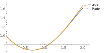
		Finally, we plot the solution along with its {5,5}-Padé approximation: pade[x_] = N[%]; s = NDSolve[{y'[x]==x^2 -(y[x])^2, y[0]==1}, y, {x,0,2}]; Plot[{pade[x],Evaluate[y[x]/.s]}, {x,0,2}, PlotRange->All, PlotLabels->{"Pade","true"}]
Padé approximation along with the rtue solution to the Riccati equation.		Mathematica code

   ■

 

References

1. Baker G.A. (1975), Essentials of Padé approximants. Academic, New York
2. John P. Boyd, Padé approximant algorithm for solving nonlinear ordinary differential equation boundary value problems on an unbounded domain, Computers in Physics, Volume 11 Issue 3, May/June 1997 Pages 299--303; https://doi.org/10.1063/1.168606
3. Gonnet, P., Güttel, S., and Trefethen, L.N., Robust Padé approximation via SVD, SIAM Review, submitted, 2011.
4. Stroethoff, K., Bhaskara’s approximation for the Sine, The Mathematics Enthusiast, 2014, Vol. 11, Issue 3, pp. 485--492.
5. Wazwaz AM (2006) The modified decomposition method and Padé approximants for a boundary layer equation in unbounded domain. Appl Math Comput 177:737–744
6. Xu H (2004) An explicit analytic solution for free convection about a vertical flat plate embedded in a porous medium by means of homotopy analysis method. Appl Math Comput 158:433–443

 

Return to Mathematica page
Return to the main page (APMA0330)
Return to the Part 1 (Plotting)
Return to the Part 2 (First Order ODEs)
Return to the Part 3 (Numerical Methods)
Return to the Part 4 (Second and Higher Order ODEs)
Return to the Part 5 (Series and Recurrences)
Return to the Part 6 (Laplace Transform)
Return to the Part 7 (Boundary Value Problems)