Preface


This section concerns about the case when a characteristic polynomial has complex conjugate roots.

Return to computing page for the first course APMA0330
Return to computing page for the second course APMA0340
Return to Mathematica tutorial for the second course APMA0340
Return to the main page for the course APMA0330
Return to the main page for the course APMA0340
Return to Part IV of the course APMA0330

Complex Roots


An exponential solution \( y = C\, e^{\lambda\,t} , \) where C ≠ 0 is an arbitrary real number and λ is a complex or real number, to the homogeneous constant coefficient linear differential equation

\begin{equation} \label{EqComplex.1} a_n y^{(n)} + a_{n-1} y^{(n-1)} + \cdots + a_1 y' + a_0 \,y = 0 , \qquad a_n \ne 0, \end{equation}
is called a modal solution and \( C\, e^{\lambda\,t} \) is called a mode of the system. If we assign to the left-hand side a linear differential operator
\begin{equation} \label{EqComplex.2} L\left[ \texttt{D} \right] = a_n \texttt{D}^n + a_{n-1} \texttt{D}^{n-1} + \cdots + a_1 \,\texttt{D} + a_0 , \qquad \texttt{D} = \frac{{\text d}}{{\text d}t} , \end{equation}
then the exponential function/mode is a solution to the homogeneous linear equation \( L\left[ \texttt{D} \right] y = 0 \) exactly when λ is a root of the characteristic equation
\begin{equation} \label{EqComplex.3} L\left( \lambda \right) = a_n \lambda^n + a_{n-1} \lambda^{n-1} + \cdots + a_1 \,\lambda + a_0 =0 . \end{equation}
If polynomial \eqref{EqComplex.3} has a simple complex root \( \lambda = \alpha + {\bf j} \beta , \) then its complex conjugate \( \overline{\lambda} = \alpha - {\bf j} \beta \) also must be a root because we consider only real-valued differential equations and all coefficients \( a_0 , a_1 , \cdots , a_n \) are assumed to be real numbers. In this case, the characteristic polynomial can be factored:
\[ L\left( \lambda \right) = a_n \left[ \left( \lambda - \alpha \right)^2 + \beta^2 \right] M \left( \lambda \right) , \qquad M \left( \alpha \pm {\bf j} \beta \right) \ne 0 . \]
Recall that L( λ ) is a real-valued polynomial of degree n and M( λ ) is a real-valued polynomial of degree n-2. If the characteristic polynomial has complex pair of roots \( \lambda = \alpha \pm {\bf j} \beta \) of multiplicity m, then it can be factored:
\[ L\left( \lambda \right) = a_n \left[ \left( \lambda - \alpha \right)^2 + \beta^2 \right]^m M \left( \lambda \right) , \qquad M \left( \alpha \pm {\bf j} \beta \right) \ne 0 , \]
where \( M\left( \lambda \right) \) is the real-valued polynomial of degree n-2m.

Now we go from the general case to analyze solutions of the second order linear differential equation with constant coefficients:

\[ a \, \ddot{y} + b\, \dot{y} + c \,y =0 , \qquad a\ne 0, \quad \ddot{y} = \frac{{\text d}^2 y}{{\text d} t^2} , \quad \dot{y} = \frac{{\text d} y}{{\text d} t} . \]
Suppose that the characteristic polynomial \( L\left( \lambda \right) = a\,\lambda^2 + b\,\lambda + c \) has a pair of complex roots:
\[ \lambda = \frac{-b \pm {\bf j} \sqrt{4ac-b^2}}{2a} , \qquad \mbox{where} \quad 4ac-b^2 >0 . \]
Recall that j is a unit vector in positive vertical direction on the complex plane so that \( {\bf j}^2 =-1 . \) Upon introducing two real numbers
\[ \alpha = -\frac{b}{2a} , \qquad \beta = \frac{\sqrt{4ac-b^2}}{2a} , \qquad \mbox{where} \quad 4ac-b^2 >0 , \]
we see that the characteristic equation \( a\,\lambda^2 + b\,\lambda + c =0 \) has two complex conjugate roots \( \lambda = \alpha \pm {\bf j} \beta . \) So the differential equation \( L\left[ \texttt{D} \right] y = 0 \) has two exponential solutions
\[ z_1 (t) = e^{\left( \alpha + {\bf j} \beta \right) t} = e^{\alpha\,t} \, e^{{\bf j} \beta\,t} , \qquad z_2 (t) = \overline{z_1 (t)} = e^{\left( \alpha - {\bf j} \beta \right) t} = e^{\alpha\,t} \, e^{-{\bf j} \beta\,t} . \]
We use the letter z here to indicate the functions are complex valued. The general solution is a linear combination of these two basic solutions:
\[ y(t) = C_1 z_1 (t) +C_2 z_2 (t) = C_1 e^{\alpha\,t} \, e^{{\bf j} \beta\,t} + C_2 e^{\alpha\,t} \, e^{-{\bf j} \beta\,t} = e^{\alpha\,t} \left[ C_1 e^{{\bf j} \beta\,t} + C_2 e^{-{\bf j} \beta\,t} \right] . \]
Because the differential equation \( L\left[ \texttt{D} \right] y = 0 \) has real coefficients, we are expecting real-valued solutions. This could be achieved only when one arbitrary constant \( C_2 = \overline{C_1} \) is complex conjugate of another one. So upon introducing two real arbitrary constants A and B such that \( 2\,C_1 = A + {\bf j} B , \quad 2\,C_2 = A - {\bf j} B , \) we get
\[ y(t) = e^{\alpha\,t} \left[ \frac{1}{2} \left( A + {\bf j} B \right) e^{{\bf j} \beta\,t} + \frac{1}{2} \left( A - {\bf j} B \right) e^{-{\bf j} \beta\,t} \right] = e^{\alpha\,t} \, \frac{A}{2} \left[ e^{{\bf j} \beta\,t} + e^{-{\bf j} \beta\,t} \right] + e^{\alpha\,t} \, \frac{B}{2} \left[ {\bf j}\,e^{{\bf j} \beta\,t} -{\bf j}\, e^{-{\bf j} \beta\,t} \right] . \]
Now we recall Euler's formula
\[ e^{{\bf j}\theta} = \cos \theta + {\bf j}\,\sin \theta, \qquad \Longrightarrow \qquad \cos\theta = \frac{1}{2} \left[ e^{{\bf j}\theta} + e^{-{\bf j}\theta} \right] , \quad \sin\theta = \frac{1}{2{\bf j}} \left[ e^{{\bf j}\theta} + e^{-{\bf j}\theta} \right] . \]
This allows us to rewrite the general solution as
\[ y(t) = e^{\alpha\,t} \, A\, \cos \left( \beta\,t \right) - e^{\alpha\,t} \, B\, \sin \left( \beta\,t \right) \]
that involve only real-valued functions. Here A and B are arbitrary real constants and the real number β is referred to as pseudo-frequency.

Theorem: : If \( z(t) \) is a complex-valued solution to

\[ L\left[ \texttt{D} \right] z = a_n \texttt{D}^n z + a_{n-1} \texttt{D}^{n-1} z + \cdots + a_1 \,\texttt{D} \,z+ a_0 \, z =0 , \qquad \texttt{D} = \frac{{\text d}}{{\text d}t} , \]
where all coefficients \( a_0 , a_1 , \ldots , a_n \) are real numbers, then the real and imaginary parts of z are also solutions.
Example: 
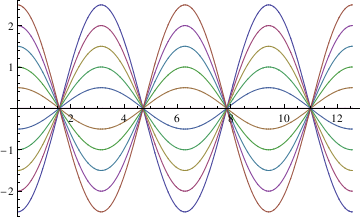
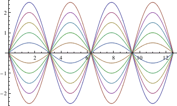
Consider second order differential equation
\[ y'' + a^2 y =0 , \qquad a>0. \]
The corresponding characteristic equation, \( \lambda^2 + a^2 =0 \) has two complex conjugate roots \( \lambda = \pm a{\bf j} , \) where j is the unit vector on the complex plane in positive vertical direction. We use Mathematica to show that the fundamental set of solutions consists of sine and cosine functions.
Clear[y]
y[t_]=c1 Cos[a*t]+c2*Sin[a*t]
Simplify[y''[t]+a^2*y[t]==0]

In this syntax, you define cosine and sine functions by Cos[ ] and Sin[ ]. When you enter the general solution, you can verify that this is indeed the solution.

Clear[y]
y[t_]=c1 Cos[a*t]+c2*Sin[a*t]

Out[7]= c1 Cos[a t] + c2 Sin[a t]
Simplify[y''[t]+a^2*y[t]==0]
Out[8]= True
Now we plot family of solutions for \( a =1 . \)
DSolve[y''[x] + y[x] == 0, y[x], x]
Out[14]= {{y[x] -> C[1] Cos[x] + C[2] Sin[x]}}
toplot1 =
Table[C[2] Cos[x] - C[1] Sin[x] /. {C[2] -> i, C[1] -> 0}, {i, -2.5, 2.5, 0.5}];
toplot2 =
Table[C[2] Cos[x] - C[1] Sin[x] /. {C[2] -> 0, C[1] -> i}, {i, -2.5, 2.5, 0.5}];
plot1 = Plot[Evaluate[toplot1], {x, 0, 4*Pi},
DisplayFunction -> Identity]

plot2 = Plot[Evaluate[toplot2], {x, 0, 4*Pi}, DisplayFunction -> Identity]
Example: We verify that the function \( y(x) = C_1 \,\cos 2x + C_2 \,\sin 2x + x^3 -3x/2 \) is a solution of the differential equation \( y'' + 4\,y = 4\,x^3 .\)

y[x_] = c1 Cos[2 x] + c2 Sin[2 x] + x^3 - 3*x/2;
Simplify[y''[x] + 4 y[x] == 4 x^3]
Out[2]= True
ics = {y[0] == 1, y'[0] == -1};
c1c2 = Solve[ics, {c1, c2}];
SolRule[x_] = y[x] /. c1c2[[1]]
SolRule''[x] + 4 SolRule[x] == 4 x^3 && SolRule[0] == 1 && SolRule'[0] == -1
Simplify[%]
Out[7]= True

To check linearly dependence:

Clear[y];
y={Cos[2 x], Sin[2 x]}
w={y,D[y,x]}
Det[w]
Out[11]= 2 Cos[2 x]^2 + 2 Sin[2 x]^2
y={x,3 x}
w={y,D[y,x]}
Det[w]
Out[15]= 0
The Euler formula:
ExpToTrig[Exp[I 2 x]]
Out[9]= Cos[2 x] + I Sin[2 x]
y={E^(a x) Cos[2x], E^(a x) Sin[2x]};
w = {y, D[y, x]};
Det[w] (* or *)
Simplify[Det[w], Trig -> True]
Out[22]= 2 E^(2 a x)
which is not zero. So these two functions are linearly independent.
Example: Consider the differential equation
\[ y'' -4\,y' + 5\, y =0 . \]
Its general solution is
\[ y= e^{2x} \left( C_1 \cos x + C_2 \sin x \right) . \]
DSolve[y''[x]-4 y'[x]+5 y[x]==0,y[x],x]
Out[1]= {{y[x] -> E^(2 x) C[2] Cos[x] + E^(2 x) C[1] Sin[x]}}
soln[x_] = Expand[y[x]/.%[[1]]]
Out[2]= E^(2 x) C[2] Cos[x] + E^(2 x) C[1] Sin[x]
y1[x_] = Coefficient[soln[x],C[1]]
Out[3]= E^(2 x) Sin[x]
y2[x_] = Coefficient[soln[x], C[2]]
Out[4]= E^(2 x) Cos[x]
Wronskian[{y1[x], y2[x]}, x] (* built-in Wronskian *)
Out[5]= -E^(4 x)
DSolve[{y''[x]-4 y'[x]+5 y[x]==0,y[0]==1},y[x],x]
Out[6]= {y[x] -> E^(2 x) (Cos[x] + C[1] Sin[x])}}

IVP:

DSolve[{y''[x] - 4 y'[x] + 5 y[x] == 0, y[0] == 1}, y[x], x];
soln[x_] = Expand[y[x] /. %[[1]]] /. C[1] -> c1
curves = Table[soln[x], {c1, -2, 2}];
Plot[Evaluate[curves], {x, -2, 2}, PlotRange -> {-10, 10}]
Out[11]= E^(2 x) Cos[x] + c1 E^(2 x) Sin[x]
Out[13]=

DSolve[{y''[x] - 4 y'[x] + 5 y[x] == 0, y'[0] == 1}, y[x], x];
soln[x_] = Expand[y[x] /. %[[1]]] /. C[1] -> c2
curves = Table[soln[x], {c2, -2, 2}];
Plot[Evaluate[curves], {x, -0.5, 2}, PlotRange -> {-10, 10}]
Out[15]= 1/2 E^(2 x) Cos[x] - 1/2 c2 E^(2 x) Cos[x] + c2 E^(2 x) Sin[x]
Out[17]=
Example: We consider the equation of motion for a mass m that is subjected to the Hookean restoring force of stiffness constant k:
\[ m \,\dot{v} = -k\,x \qquad \Longrightarrow \qquad \frac{\text d}{{\text d}t} \, \frac{v}{\omega_0} = - \omega_0 x , \]
where \( \omega_0 = \sqrt{k/m} \) is the angular frequency of the motion. Next, we rewrite the equation for the instantaneous velocity as
\[ \frac{\text d}{{\text d}t} \, x = \omega_0 \left( \frac{v}{\omega_0} \right) . \]
Upon adding this equation to the equation of motion with multiple j, the unit vector in positive vertical direction on the complex plane ℂ, we obtain
\[ \frac{\text d}{{\text d}t} \left( x + {\bf j}\,\frac{v}{\omega_0} \right) = \omega_0 \left( \frac{v}{\omega_0} - {\bf j} \,x \right) = -{\bf j}\,\omega_0 \left( x + {\bf j} \,\frac{v}{\omega_0} \right) . \]
Finally define
\[ z = x + {\bf j} \,\frac{v}{\omega_0} , \]
we get
\[ \frac{\text d}{{\text d}t} \, z = -{\bf j}\,\omega_0 z , \]
which is a first order differential equation for the complex quantity z. The above equation for z is separable, so we integrate it directly:
\[ \frac{{\text d}x}{z} = -{\bf j}\,\omega_0 \,{\text d}t \qquad \Longrightarrow \qquad z(t) = z_0 e^{-{\bf j}\,\omega_0 t} , \]
where \( \displaystyle z_0 = x_0 + {\bf j}\, \frac{v_0}{\omega_0} \) is the initial quantity. Now we immediately derive
\[ x + {\bf j} \,\frac{v}{\omega_0} = \left( x_0 + {\bf j}\, \frac{v_0}{\omega_0} \right) e^{-{\bf j}\,\omega_0 t} . \]
This formula represents the general solution of the equation of motion for the oscillator: the instantaneous position and velocity of the particle are equal to the real part and to ω0 times the imaginary part of the complex quantity z.

Taking the magnitude of both sides of complex quantity z, we have

\[ x^2 + \frac{v^2}{\omega_0^2} = x^2_0 + \frac{v^2_0}{\omega_0^2} = A_0^2 \]
is a constant over time. We can rewrite this relation in terms or energy components:
\[ \frac{1}{2} \, m\,v^2 + \frac{1}{2}\, k\, x^2 = \frac{1}{2}\, k\, A_0^2 , \]
where A0 is the constant amplitude of the motion and
\[ \phi = \arctan \left( \frac{v_0}{\omega_0 x_0} \right) \]
is the phase of the complex quantity z0. Then we have
\[ x + {\bf j} \,\frac{v}{\omega_0} = A_0 e^{{\bf j} \left( \phi - \omega_0 t \right)} , \]
whose real part gives the position of the mass:
\[ x (t) = A_0 \cos \left( \phi - \omega_0 t \right) . \]
      ▪
Example: It is possible to extend the previously considered example for the case when damping term is modeled by a linear expression proportional to the velocity:
\[ m\,\dot{v} = -k\,x - \gamma m\,v . \]
Upon division by the trouble maker m, we get
\[ \frac{\text d}{{\text d}t}\, v = -\omega_0^2 x - \gamma\, v , \]
where \( \omega_0 = \sqrt{k/m} . \) Let
\[ x(t) = e^{\lambda t}\, u(t) , \]
then for u we have
\[ \left[ \lambda^2 u + 2\lambda\,\frac{{\text d}u}{{\text d}t} + \frac{{\text d}^2 u}{{\text d}t^2} \right] e^{\lambda t} = -\omega_0^2 u\,e^{\lambda t} - \gamma \left[ \lambda \,u + \frac{{\text d}u}{{\text d}t} \right] e^{\lambda t} . \]
After some minor rearrangements and setting 2λ = -γ, we obtain
\[ \frac{{\text d}^2 u}{{\text d}t^2} = - \omega^2 u , \]
where
\[ \omega = \sqrt{\omega_0^2 - \frac{\gamma^2}{4}} = \sqrt{\frac{k}{m} - \frac{\gamma^2}{4}} \]
is a damped angular frequency. Upon introducing a new dependent variable
\[ w = \frac{{\text d}u}{{\text d}t} , \]
one can rewrite the above equation as
\[ \frac{{\text d}}{{\text d}t} \,\frac{w}{\omega} = - \omega\, u . \]
Now similar to the previous example, we introduce a complex quantity
\[ z = u + {\bf j}\, \frac{w}{\omega} \qquad \Longrightarrow \qquad \frac{{\text d}}{{\text d}t} \,z = -{\bf j}\omega \,w . \]
Its solution is readily found to be
\[ z(t) = u(t) + {\bf j}\, \frac{w(t)}{\omega} = \left( u_0 + {\bf j}\, \frac{w_0}{\omega} \right) e^{-{\bf j}\omega t} = A_0 e^{{\bf j}\left( \theta -\omega t \right)} , \]
where
\[ A_0 = \sqrt{u_0^2 + \frac{w_0}{\omega}} \qquad\mbox{and} \qquad \theta = \arctan \left( \frac{w_0}{\omega}\, u_0 \right) . \]
Extracting the real part, we find the general solution to be
\[ x(t) = e^{-\gamma t/2} u(t) = e^{-\gamma t/2} \,A_0 \, \cos \left( \theta -\omega t \right) . \]
      ▪


Equations with complex coefficients


So far, we discussed differential equations with real coefficients. Now we turn to complex coefficient case that is also important. WE present this topic through examples.
Example: Let us consider the initial value problem on semi-infinite interval (-∞,0):
\[ w'' -2{\bf j}\pi^2 w(z) = 0, \qquad \lim_{z\to -\infty} =0 , \quad w' (0) = {\bf j}\,a , \]
where 𝑎 is a positive real number. First, we ask Mathematica to find the general solution to the given second-order linear differential equation
sol = DSolve[-2 I \[Pi]^2 w[z] + w''[z] == 0, w[z], z] // ExpToTrig // ComplexExpand
{{w[z] -> C[1] Cos[\[Pi] z] Cosh[\[Pi] z] + C[2] Cos[\[Pi] z] Cosh[\[Pi] z] + C[1] Cos[\[Pi] z] Sinh[\[Pi] z] - C[2] Cos[\[Pi] z] Sinh[\[Pi] z] + I (C[1] Cosh[\[Pi] z] Sin[\[Pi] z] - C[2] Cosh[\[Pi] z] Sin[\[Pi] z] + C[1] Sin[\[Pi] z] Sinh[\[Pi] z] + C[2] Sin[\[Pi] z] Sinh[\[Pi] z])}}
Now let us take its limit as z → -∞ in two cases when one of arbitrary constants is zero:
Limit[w[z] /. sol /. {C[1] -> 0}, z -> -\[Infinity]]
{ComplexInfinity}
Limit[w[z] /. sol /. {C[2] -> 0}, z -> -\[Infinity]]
{0}
Therefore, we have to set C[2] = 0. Now we determine C[1] to satisfy the boundary condition at z = 0:
Solve[(D[(w[z] /. sol /. C[2] -> 0), z] /. z -> 0) == I*a, C[1]]
{{C[1] -> ((1/2 + I/2) a)/\[Pi]}}
This gives us the required solution
\[ w(z) = \frac{a}{2\pi} \left( 1 + {\bf j} \right) \left[ \cos (\pi z)\,\cosh (\pi z) + \cos (\pi z)\, \sinh (\pi z) + \sin (\pi z) \,\cosh (\pi z) + \sin (\pi z) \,\sinh (\pi z) \right] . \]
What if some linear combination of the coefficients is zero, but both C[1] and C[2] are non-zero? Then you can't find the solution by testing simple cases. In this particular problem we are lucky: the correct boundary condition at infinity is C[2]==0 instead of Pi C[1]-4 C[2]== 0 or something.

We proceed without ComplexExpand

generalsol = DSolve[{-2 I \[Pi]^2 w[z] + w''[z] == 0, w'[0] == (I a)}, w[z], z]
((1/2 - I/ 2) E^((-1 - I) \[Pi] z) (-I a + (1 + I) \[Pi] C[ 1] + (1 + I) E^((2 + 2 I) \[Pi] z) \[Pi] C[1]))/\[Pi]
the output expression is not suitable for elimination of one of the arbitrary constants because the solution contains complex exponents. To make the coefficient clearer, we type
Collect[generalsol, Exp[_], Simplify]
E^((1 + I) \[Pi] z) C[1] + E^((-1 - I) \[Pi] z) (-(((1/2 + I/2) a)/\[Pi]) + C[1])
Apparently, the coefficient of the divergent exponent must be zero:
\[ \frac{a}{2\pi} \left( 1 + {\bf j} \right) + C_1 = 0. \]
Then
sol = Function[z, #] &[ E^((1 + I) π z) C[1] /. C[1] -> ((1/2 + I/2) a)/(π)]
Function[z, ((1/2 + I/2) a E^((1 + I) \[Pi] z))/\[Pi]]
We check our answer with Mathematica:
{-2 I π^2 w[z] + w''[z] == 0, w[-∞] == 0, w'[0] == 0 + (I a)} /. w -> sol // Simplify
{True, True, True}
      ▪


  1. Gauthier, N., Novel approach for solving the equation of motion of a simple harmonic oscillator, International Journal of Mathematical Education in Science and Technology, 2004, Vol. 35, No. 3, pp. 446--452. https://doi.org/10.1080/00207390410001686580
  2. Kobayashi, Y., A geometrical key to solution of differential equation: d^{2}x(t)/ dt^{2} &eq; - ω² x(t)'', The Mathematical Gazette, 2003, Vol. 87, pp. 163--166.
  3. Weinstock, R., Laws of Classical Motion: What's F? What's m? What's a?, American Journal of Physics, 1961, Vol. 29, Issue 10, pp. 698. https://doi.org/10.1119/1.1937555
  4. Weinstock, R., An unusual method of solving the harmonic-oscillator equation, American Journal of Physics, 1961, Vol. 29, Issue 12, pp. 830--831; https://doi.org/10.1119/1.1937628


Return to Mathematica page
Return to the main page (APMA0330)
Return to the Part 1 (Plotting)
Return to the Part 2 (First Order ODEs)
Return to the Part 3 (Numerical Methods)
Return to the Part 4 (Second and Higher Order ODEs)
Return to the Part 5 (Series and Recurrences)
Return to the Part 6 (Laplace Transform)
Return to the Part 7 (Boundary Value Problems)