Return to computing page for the second course APMA0340
Return to Mathematica tutorial for the second course APMA0340
Return to the main page for the course APMA0330
Return to the main page for the course APMA0340
Return to Part IV of the course APMA0330
Glossary
Preface
There are several reasons to study second and higher order differential equations. Most dynamic models in mechanics (including quantuum) involve second order differential equations because their formulations involve either Newton's second law of Euler--Lagrange formalism.
There are many problems that lead to the differential equation of the form
|
|
|
|

|
|
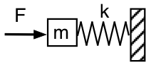
All these dodels lead to a simple harmonic oscillator upon linearization:
Second and Higher Order Differential Equations
This chapter is devoted to differential equations of order higher than one. Of course, the first question that comes to your mind: why? After some further thoughts, you should probably realize that these equations constitute a significant part of tools needed to model real world, and you may recall from school Newton's second law: `` A change in motion is proportional to the motive force impressed and takes place along the straight line in which that force is impressed (Isaac Newton).'' Its common form is \( {\bf F} = m{\bf a} , \) where m is the mass and a is the acceleration: \( {\bf a} = {\text d}{\bf v}/{\text d} t = {\text d}^2 {\bf x} / {\text d} t^2 , \) which is expressed as the second derivative of the displacement, x. A change in velocity v must be accompanied by a force affecting every part of the body.
Ordinary differential equations (ODEs) may be divided into two classes: linear equations and nonlinear equations. The latter have a richer mathematical structure than linear equations and generally more difficult to solve in closed form. Unfortunately, the techniques applicable for solving second order nonlinear ODEs are not available at an undergraduate level. Therefore, we concentrate our attention on linear differential equations. However, some nonlinear equations will be exposed later to demonstrate modeling of real world phenomena. Also, we present some classes of nonlinear equations that can be reduced to the first order differential equations.
Linear differential equations of second order are of crucial importance in the study of differential equations for two main reasons. First of all, linear equations have a rich theoretical structure that underlies a number of systematic methods of solutions. Further, a substantial portion of this structure and of these methods is understandable at a fairly elementary mathematical level. The second reason to study second order linear equations is that they are vital to any serious investigation of the classical areas of mathematical physics.
For a general n-th order differential equation, \( \displaystyle F\left( x, y, y' , \ldots , y^{(n)} \right) = 0 , \) its general solution is a solution containing n arbitrary independent constants from some domain in ℝn.
Theorem: Suppose \( f\,:\,\mathbb{R}^3 \mapsto \mathbb{R} \) is continuous in some cube |x - x0| ≤ 𝑎, |y - α| ≤ b, |v - β| ≤ c and that the partial derivatives \( \partial f(x,y,v)/\partial y \) and \( \partial f(x,y,v)/\partial v \) are also continuous there. Then there is some interval \( \left\vert x - x_0 \right\vert \le h \le a \) in which the initial value problem
Motivation to use higher order derivatives
Usually, we are exposed to a wide variety of external motion and movement on a daily basis. From driving a car to catching an elevator, our bodies are repeatedly exposed to external forces acting upon us, leading to acceleration. Excluding the force of gravity to which we all are accustomed, the accelerations that we normally experience are not constant. When we are in a car and accelerate as the lights change to green, our acceleration is not constant. Our body does not feel velocity, but only the change of velocity i.e., acceleration, brought about by the force exerted by an object on our body. We are going to illustrate the concepts with practical examples of parachute problem, roller coasters, and trampolines.
There is no universal agreement of the names of higher order derivatives. We use the term jerk for the third derivative and snap to denote the fourth derivative of displacement with respect to time. The fifth and sixth derivatives with respect to time are referred to as crackle and pop, respectively. The origin of the use of the term jerk to denote the time rate of change of acceleration is obscure. The French geometer Transon (A. Transon, Journal de Mathématiques Pures et Appliquées, vol. 10, 320, 1845) was probably the first to consider the third time derivative of distance in mechanics and he uses the term virtualite for it. The concept of the jerk, as a predictor of large accelerations of short duration, has important practical engineering applications in the design of intermittent-motion mechanisms such as cams (they turn rotary motion into reciprocating motion) and genevas (one of the most commonly used devices for producing intermittent rotary motion, characterized by alternate periods of motion and rest with no reversal in direction), as well as in design of the transition curves that provide a gradual rise in curvature from straight paths to circular arcs in railways and highways.
Acceleration without jerk is just a consequence of static load. Jerk is felt as the change in force, similar when one opens the parachute during free fall. Acceleration of a paratrooper does not suddenly switch on, but instead grows from one value to another during a short period of time. So there must be some jerk involve (which may be very significant). Changing jerk involves some snap. This can be expressed mathematically as
Let the motion of a particle along a three times continuously differentiable plane curve C be described as a function of time t by the position vector r(t) measured from a given fixed origin. Let the curve C be given in the intrinsic form \( \rho = \rho (s) , \) where s is arc length measured from a given fixed point on C and ρ is the radius of curvature at any point of the path. Then the velocity vector v(t) and vector acceleration a(t) can be expressed in the tangential-normal form:
The time rate of change of the vector acceleration is called the vector jerk and is obtained by differentiating the acceleration and using \( \dot{\bf t} = \left( v/\rho \right) {\bf n} \) and \( \dot{\bf n} = -\left( v/\rho \right) {\bf t} . \) The result is
An area conservation law in the hodograph plane can be deduced similar to that which holds for the position vector in planar motion under a central force. If dφ denotes the angle between the velocity vector v at time t and a neighboring velocity vector v + dv at time t + dt, then the sectorial area dA along the hodograph between v and v + dv is given by
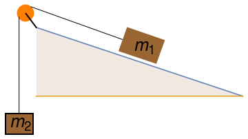
disk = Graphics[{Orange, Disk[{-0.3, 2.4}, 0.25]}];
line = Graphics[{Thick, Black, Line[{{-0.3, 2.4}, {0, 2}}]}];
rectangle2 = Graphics[{EdgeForm[Thick], Brown, Rectangle[{-0.9, -1.1}, {-0.1, -0.5}]}];
line2 = Graphics[Line[{{-0.5, 2.3}, {-0.5, -0.5}}]];
polygon = Graphics[{Brown, Polygon[{{2.4, 1.3}, {2.65, 2.0}, {3.75, 1.62}, {3.5, 0.93}}]}];
line1 = Graphics[Line[{{-0.15, 2.6}, {2.5, 1.65}}]];
m1 = Graphics[ Text[Style["\!\(\*SubscriptBox[\(m\), \(1\)]\)", Large], {3.15, 1.5}]];
m2 = Graphics[ Text[Style["\!\(\*SubscriptBox[\(m\), \(2\)]\)", Large], {-0.45, -0.73}]];
Show[disk, ramp, line, rectangle2, line2, line1, polygon, m1, m2]
- Abell, M.L., and Braselton, J.P., Differential Equations with Mathematica, Fourth edition, Elsevier, Boston, 2020.
- Enns, Richard H. and McGluire, George C., Nonlinear Physics with Mathematica for Scientists and Engineers, Birkhäuser, Boston, 2001.
- Hoensch, Ulrich, A., Differential Equations and Applications Using Mathematica,
- Kamke, E., Handbook on Ordinary Differential Equations, Chelsea Publ., Leipzig, 1974.
- Lynch, Stephen Dynamical Systems with Applications Using Mathematica, Birkhäuser (2007), 484 pp., 2007.
- Noonburg, Virginia W., Differential Equations: From Calculus to Dynamical Systems, Second edition, MAA Press, 2019.
- Polyanin, A.D., Zaitsev, V.F., in: Handbook of Exact Solutions for Ordinary Differential Equations, second ed., Chapman & Hall/CRC, Boca Raton, 2003.
- Zwillinger, Daniel, and Dobrushkin, Vladimir, Handbook of Differential equations, Fourth edition, CRC Press, Boca Raton, 2021.
Return to Mathematica page
Return to the main page (APMA0330)
Return to the Part 1 (Plotting)
Return to the Part 2 (First Order ODEs)
Return to the Part 3 (Numerical Methods)
Return to the Part 4 (Second and Higher Order ODEs)
Return to the Part 5 (Series and Recurrences)
Return to the Part 6 (Laplace Transform)
Return to the Part 7 (Boundary Value Problems)