This section is devoted to a fascinating method for solving linear and nonlinear ordinary and partial
differential equations invented by George Adomian (1922--1996). This method
will be used in some other sections, so here we just give it a friendly introduction.
Return to computing page for the first course APMA0330
Return to computing page for the second course APMA0340
Return to Mathematica tutorial for the first course APMA0330
Return to Mathematica tutorial for the second course APMA0340
Return to the main page for the course APMA0330
Return to the main page for the course APMA0340
The Adomian decomposition method (ADM) is a systematic approximation method for solving nonlinear functional equations including ordinary and partial differential equations. It was named by Richard Bellman in honor of Adomian because it was developed from the 1970s --- 1990s by an American mathematician and aerospace engineer of Armenian descent George Adomian (1922-1996), chair of the Center for Applied Mathematics at the University of Georgia. The method is based on the assumption that the solution to a nonlinear functional equation can be represented by the infinite series \( y(x) = \sum_{n \ge 0} u_n (x) . \) The crucial aspect of the method is the decomposition of the problem under consideration into a sequence of recursively specified auxiliary problems that can be solved explicitly. This stage utilizes the employment of so called "Adomian polynomials" to represent the nonlinear portion of the equation as a convergent series with respect to these polynomials, without actual linearization of the system. These polynomials were named after G. Adomian by Randolph Rach in 1984 (A convenient computational form for the Adomian polynomials can be found in the Journal of Mathematical Analysis and Applications, Volume 102, Issue 2, September 1984, pages 415--419).
There are several known algorithms for calculating Adomian polynomials; the following publications reflect efforts made in this area:
Babolian, E. and Javadi, Sh., “New method for calculating Adomian polynomials”, Applied Mathematics and Computation, 2004, Volume 153, Issue 1, 25 May 2004, pages 253--259. https://doi.org/10.1016/S0096-3003(03)00629-5
Biazar, J., Babolian, E., Kember, G., Nouri, A., Islam, R., An alternate algorithm for computing Adomian polynomials in special cases, Applied Mathematics and Computation, 2003,
Volume 138, Issues 2–3, 20 June 2003, Pages 523--529;
https://doi.org/10.1016/S0096-3003(02)00174-1
Chen, W., and Lu, Z., An algorithm for Adomian
decomposition method, Applied Mathematics and Computation, 2004, Vol. 159, No. 1, (2004) pp. 221--235.
Choi, H.-W., and Shin, J.G., Symbolic implementation of the algorithm for calculating Adomian polynomials, Applied Mathematics and Computation, 2003, Volume 146, Issue 1, 30 December 2003, Pages 257--271; https://doi.org/10.1016/S0096-3003(02)00541-6
Fatoorehchi, H. and Abolghasemi, H. (2011b), “On calculation of Adomian polynomials by MATLAB”, Journal of
Applied Computer Science and Mathematics (“Stefan cel Mare” University of Suceava), 2011, Vol. 11, No. 5, pp. 85--88.
Liao, S.J., On the homotopy analysis method for nonlinear problems, Applied Mathematics and Computation, 2004, Vol. 147, Issue 2, pp. 499--513; https://doi.org/10.1016/S0096-3003(02)00790-7
Rach, R.C., “A new definition of the Adomian polynomials”, Kybernetes, Vol. 37 Issue: 7, 2008, pp.910--955, https://doi.org/10.1108/03684920810884342
Wazwaz, A.M., A new algorithm for calculating Adomian polynomials for non-linear operators, Applied Mathematics and Computation, 111 (2000), pp. 53--69.
Let me introduce some scientists (in alphabetic order) who
contributed to and greatly improved the Adomian Decomposition Method
to make it available to the mathematical and engineering community.
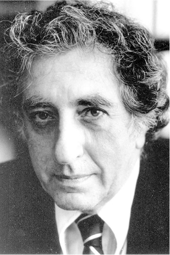
George Adomian
Dr. George Adomian (1922--1996) was an American mathematician, theoretical physicist, and electrical engineer of Armenian descent. He received his Ph.D. degree from UCLA. He first proposed and considerably developed the Adomian Decomposition Method (ADM) for
solving nonlinear differential equations, both ordinary, and partial,
deterministic and stochastic, also integral equations, algebraic and
transcendental (functional), and matrix equations. He was a
Distinguished Professor (academic rank), the David C. Barrow Professor
of Mathematics (Chair), and the Director of the Center for Applied
Mathematics at the University of Georgia, the founder and Chief
Scientist of General Analytics Corporation, a winner of the 1989
Richard Bellman Prize for outstanding contributions to nonlinear
stochastic analysis, and a 1988 National Academy of Sciences Scholar.
He is the author of eight books and over three hundred journal papers.
Dr. Adomian was the Radar Officer (naval rank of Lieutenant, the
equivalent of a Captain in the Army by direct commission) aboard the
USS Antietam (CV-36), and served in the Pacific Theater of Operations
during the Second World War. He also attended the secret radar school
at MIT that trained the first radar officers for the U.S. Navy.
His obituary was prepared by Randolph Rach and appears in
R. Rach, Dr. George Adomian – distinguished scientist and
mathematician, Kybernetes, Vol. 25, No. 9, 1996, 45-50.
Yves Cherruault
Dr. Yves Cherruault (1937--2010) was a French mathematician. He received his Ph.D. degree from the University of Paris. He was a professor of mathematics at the University Pierre et Marie Curie, Paris, and the Director of MÉDIMAT (Laboratory of Mathematics Applied to Biomedicine). Professor Cherruault is one of the founders of the field of Biomathematics and an author of seven books and over two hundred journal papers. Dr. Cherruault developed some of the convergence theorems of the ADM.
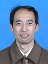
Jun-Sheng Duan
Dr. Jun-Sheng Duan is a Chinese applied mathematician and computer scientist born in Inner Mongolia, China, in 1965. He received his Ph.D. degree from Shandong University, China. He has made extensive contributions to solutions of differential equations in mathematical physics and engineering using ADM and the Modified Decomposition Method (MDM) in collaboration with Drs. Rach and Wazwaz. He has been a professor of mathematics at the Inner Mongolia Polytechnic University, the Tianjin University of Commerce, and currently at the School of Sciences, Shanghai Institute of Technology, China. He is the author of more than eighty journal papers. Dr. Duan is an outstanding player of wei qi (the Chinese “game of go”), and ping-pong (table tennis). He enjoys photography and traveling.
Randolph Rach
Dr. Randolph Rach is a retired Army veteran and former Senior Engineer at Microwave Laboratories Inc. His experience includes research and development in microwave electronics and traveling-wave tube technology, and his research interests span nonlinear system analysis, nonlinear ordinary and partial differential equations, nonlinear integral equations and nonlinear boundary value problems. He published more than one hundred and thirty papers in applied mathematics, and he is an early contributor to the ADM. Dr. Rach’s fundamental theorems established the basis for the early development of ADM. He was also the first to propose the modified decomposition method (MDM for short). His past and current research continue to advance ADM/MDM work. He prepared the comprehensive bibliography on ADM:
R. Rach, A bibliography of the theory and applications of the Adomian
decomposition method, 1961-2011, Kybernetes, Volume 41, Nos. 7/8,
2012, 1087--1148.
Sergio E. Serrano
Dr. Sergio E. Serrano was born in Santander (Colombia) in 1953. He is a professor of environmental engineering, hydrologic science, applied mathematics,
and philosophy at Temple University in Philadelphia. He received his Ph.D. degree at the University of Waterloo (Canada). He has more than one hundred research
publications in international science, engineering, and mathematical journals. He is also the author of eight books in environmental engineering, statistics,
philosophy, and psychology. Dr. Serrano has been awarded four times with nationally-competitive research grants by the National Science Foundation, Washington,
DC. Using adaptations and modifications of the ADM, he has developed hundreds of practical engineering models of flood wave propagation, contaminant transport, and
groundwater flow in irregular geometries. He published influential textbooks on applications of differential equations in CAS Maple and Hydrology:
Sergio E. Serrano, Differential Equations, HydroScience Inc. Amber, Pennsylvania, 2016, ISBN 97809888865211
Sergio E. Serrano, Hydrology for Engineers, Geologists, and Environmental Professionals. An Integrated Treatment
of Surface, Subsurface, and Contaminant Hydrology. HydroScience Inc., Ambler, PA.
Dr. Serrano has a passion for hiking. In 1973, he explored the rain forest of the Darien Sierra on foot from Acandi (Colombia) to Yaviza (Panama). He plays the recorder (Renaissance flute). He enjoys alchemy, archaeology, home wine making, herbal medicine, and cooking. He believes that the joy of meaningful living and meaningful relationships can be found in the simplicity of everyday life. He lives in Philadelphia with his wife of thirty years and his daughter.
Abdul-Majid Wazwaz
Dr. Abdul-Majid Wazwaz is a Professor of Mathematics at Saint Xavier University in Chicago. He received his Ph.D. from the University of Illinois at Chicago. He was the author and co-author of more than four hundred and fifty papers in applied mathematics and mathematical physics. He is the author of five books on the subjects of discrete mathematics, integral equations, and partial differential equations. He has contributed extensively to theoretical advances in solitary waves theory, the ADM, and other computational methods. He is a member of the editorial board of the journals Nonlinear Dynamics (Springer) and Physica Scripta (IOP). For three years in a row, 2014, 2015, and 2016, Thomas Reuters granted him three different badges for being a “Highly Cited Researcher.”
The Adomian decomposition method (ADM for short) has led to several
modifications on the method made by various researchers in an attempt
to improve the accuracy or expand the application of the original
approach. Obviously, this tutorial cannot cover and explain all available improvements for the method. Instead,
we show how the Adomian's decomposition method works in a series of
examples. The basic spirit of the decomposition method consists of three
steps.
The first one includes a decomposition of the true solution to the initial value problem (or boundary value problem) into the infinite sum of the solution's components to auxiliary problems.
The second step asks to find the solution's components recursively based on previously obtained components, so it involves solution of a full-history recurrence. This stage requires solving very basic differential equations with explicitly determined right-hand side expressions that are obtained by decomposition of nonlinear terms into the so called Adomian's polynomials.
Finally, summation of the first finite number of components leads to an approximation to the true solution with any desired level of high precision.
If the given differential equation is homogeneous (without
a driving term), then the ADM finite sum always provides the truncated series version to the true solution provided that the Adomian series converges. However, for inhomogeneous differential equations, the ADM finite sum approximation may include some noise terms that eventually are canceled out with subsequent iterations assuming that
all iterations are complete. This phenomenon is well-known for Picard's iteration. Unwanted terms in the ADM applications were first discovered by G. Adomian and R. Rach in 1986 (The noisy convergence phenomena in decomposition method solutions,
Journal of Computational and Applied Mathematics, Volume 15, Issue 3,
July 1986, pages 379--381).
Although it is
possible to reduce these unwanted noise terms, as shown by Abdul-Majid
Wazwaz and other researchers, the issue remains. However, these
noise terms usually do not effect the approximations because they are rapidly damped out numerically.
The first proof of convergence of the ADM was given by Cherruault in 1989, who used fixed point theorems for abstract functional equations. Since conditions of these theorems are too restrictive for most physical and engineering applications to be verified in practice, many other articles on convergence of the ADM were published. In spite of the variety of publications on convergence, computational complexity, improvements, and applications of the ADM, no precise criterion of convergence was formulated in the literature, at least in the context of initial-value problems for ordinary and partial differential equations. When the slope function is a holomorphic function, then the formalism of the Cauchy--Kowalevskaya
theorem guarantees that solutions of initial-value problems for systems of ordinary differential equations exist and are analytic for small time intervals. Recent reviews on this topic can be found in the following articles: Ray's (New Approach for General Convergence of the Adomian Decomposition Method, World Applied Sciences Journal, 2014, Vol. 32, No. 11, pp. 2264--2268), Rach's (Bougoffa, L., Rach, R.C., El-Manouni, S., A convergence analysis of the Adomian decomposition method for an abstract Cauchy problem of a system of first-order nonlinear differential equations, International Journal of Computer Mathematics, 2013,
Volume 90, Issue 2, pages 360--375), and Sunday's (Convergence analysis and implementation of Adomian
decomposition method on second-order oscillatory problems, Asian Research Journal of Mathematics, 2017, Vol. 2, No. 5, pp. 1--12. Article no.ARJOM.32011) articles.
Let us compare the ADM and Picard's iteration scheme. The latter can be successfully applied only for differential equations with polynomial slope functions. The ADM extends Picard's requirements for analytically defined nonlinearities. The advantage of
Adomian’s method over the Picard scheme is the ease of computation of
successive terms. At each iterative step, the Adomian decomposition
method actually requires solving the same (very simple) initial
value problem with homogeneous initial conditions. Since
the ADM presents the solution as (infinite) series, it avoids
repetitions that slow down Picard's procedure. Although it is a
challenging problem to explicitly determine the radius of convergence for the
solution obtained on the basis of the ADM, it is usually much larger
than that of Picard's prediction.
These advantages of the ADM over Picard's iteration scheme are
abated by preprocessing: one should evaluate Adomian's polynomials
that are used at every iteration step. The labor involved in such
evaluation grows exponentially in general. This drawback becomes
negligible in an explicit one step numerical implementation based on
the ADM when only a few first terms are taken into account. It should
be noted that the amount of work for the ADM preprocessing is larger than, say, the well known
Runge--Kutta or cubic spline algorithms where a user enters only the slope
functions and the initial conditions. Usually, the labor required by ADM preprocessing is compensated by a larger step size
in the computations
than in standard one step algorithms.
We start a demonstration of the Adomian decomposition method with the
following initial value problem:
\[
y' = f(x,y) + g(x), \qquad y(x_0 ) = y_0 ,
\]
where f is the given (smooth) function, g is an input
(driving) term, y is the (unknown) output of the system, and
constants x0 and y0 are
prescribed. According to the ADM, we seek an approximation to the
solution of this initial value problem as an infinite series of
functions un to be determined recursively:
which is actually
the Faà
di Bruno's formula applied to the composition of two
functions: f and \( \sum_{k\ge 0} u_k . \)
These polynomials were first introduced by G. Adomian and R. Rach in their 1983 paper (Inversion of nonlinear stochastic operators,
Journal of Mathematical Analysis and Applications, Vol. 91, No. 1,
January 1983, pp. 39--46).
In the preceding formula, the parameter λ is a grouping parameter
that is used to identify a certain iteration term. The coefficient of
λn corresponds to the nth iteration term. One of the
ways to extract this term is to differentiate n times the
composition \( f \left( x, \sum_{k\ge 0} u_k
\lambda^k \right) \)
and set λ = 0 to eliminate the rest of the terms. Note that the previous
terms are eliminated by
differentiation. Fortunately, Mathematica has two dedicated
commands for extracting coefficients from a
polynomial: Coefficient that gives a particular coefficient
and CoefficientList that provides all coefficients of
the given polynomial (but not an arbitrary function).
The Adomian decomposition method assumes that the solution to the given initial value problem
where the An are Adomian's polynomials. To derive the expression for these polynomials, we consider the Taylor expansion of the slope function about u0:
\[
f(x,y) = f(u_0 ) + f' (u_0 ) \left( y - u_0 \right) + \frac{1}{2!}\, f''
(u_0 ) \left( y - u_0 \right)^2 + \frac{1}{3!}\, f^{(3)} (u_0 ) \left( y - u_0 \right)^3 + \cdots + \frac{1}{n!}\, f^{(n)} (u_0 ) \left( y - u_0 \right)^n + \cdots ,
\]
where we dropped writing the independent variable for simplicity because it does not affect the derivation. Substituting this expansion into the solution series and noting that
To calculate the first Adomian polynomial A0, consider any term where the sum of the subscripts of the ui add up 0. Next to get A1, consider each term where the subscripts of the ui add up 1. In a similar fashion, the general Adomian polynomial An includes any term where the sum of the subscripts of the ui add up to n.It is worth noting that the sum of the subscripts of the term uij is ij and not i.
▣
There are several known modifications of the Adomian polynomials, but we
will use only one, known as accelerated Adomian polynomials (since there is no standard notation, we denote them by aAn) that were
first introduced by George Adomian in his 1989 book (Nonlinear Stochastic Systems Theory and Applications to Physics, Kluwer Academic Publishers, Dordrecht):
In general, since the Adomian method requires the existence of all derivatives (holomorphy) for the slope function, which is more restrictive than the Lipschitz condition required for Picard's procedure, it is expected that the ADM converges faster than its Picard counterpart.
The initial term u0 in the series expansion \( y(x) = \sum_{n \ge 0} u_n (x) \) is a solution of the truncated initial value problem:
\[
y' = g(x), \qquad y(x_0 ) = y_0 ,
\]
because it incorporates the influence of all inhomogeneous terms of the problem (that includes the initial condition and the forcing input function g). Once it is achieved, all other terms in the infinite series are solutions of the homogeneous initial value problems.
Therefore, u0 is usually not the same initial approximation as in Picard's iteration procedure that is just the initial value y0. It should be noted that when the Adomian method is applied to other problems (not necessarily initial value problems for first order differential equations as we consider in this section) one can choose another approximation to the nonhomgeneous differential equation: it is important to exclude, depending on x, the input term from the given slope function.
So in this section, we follow the standard ADM procedure applicable to differential equations of the form: \( y' = f(x,y) + g(x) . \)
Therefore, the initial term u0 could be chosen with some flexibility. Once u0 is determined, all other terms in Adomian's decomposition follow from the recursive initial value problems of Appell's type:
Note: Adomian polynomials are not polynomials in the variable x. They are only polynomials in u1, … ,un, but not in u0. Additionally, components u1, … ,un might not be polynomials in the variable x.
Adomian's polynomials can be evaluated using the Duan's code (Applied Mathematical Modelling, 2013, 37, Issues 21-22, pp. 8687--8708) as follows:
Example:
Let us consider the nonlinear (pendulum) operator: \( N\left[ \theta \right] = \sin\theta . \) Then the first few Adomian's polynomials for this nonlinear operator are
and so on.
Let us consider the hyperbolic sine nonlinear function \( N\left[ x \right] = \sinh \left( x/2 \right) . \) The corresponding Adomian's polynomials are
and so on.
Our next example is the power function: \( N\left[ u \right] = u^{\gamma} , \) where γ is a real number. Then corresponding Adomian's polynomials are
Example:
Consider the simplest algebraic equation---the quadratic equation
\[
a\,x^2 + b\,x + c = 0, \qquad b\ne 0,
\]
where 𝑎, b, and c are some given constants. The case b = 0 can be easily included in our consideration by adding and subtracting the x term. The idea of isolating x is to transform the given problem to the form x = Φ(x), with some continuous function Φ, so that it appears as a fixed point problem. From the given quadratic equation, we obtain
In general, one can add and subtract k x, k ≠ 0, and express x as
\[
x = -\frac{c}{k} + \frac{k-b}{k}\, x - \frac{a}{k}\, x^2 = \alpha + \beta\, x + \gamma \,x^2 \qquad (k \ne 0).
\]
In our case, we have k = b, but later we will consider other values of k.
It is helpful to work a numerical example and show all calculations for it. Hence, we consider the equation
\[
x^2 - x -6 =0,
\]
whose solutions are known to be x = 3 and x = -2. Let us see how ADM arrives at these values. We rewrite our quadratic equation in the form suitable for the fixed point theorem
The series converges when \( \left\vert 4\alpha \gamma /\beta^2 \right\vert < 1 . \) So the series converges when
\( b^2 > |a\,c| . \) This condition is violated for our case and the Adomian series diverges. We can see this by finding derivatives of f(x) = x² - 5 at the roots:
\( f' (3) = 2\,(3) = 6 > 1 \) and \( f' (-2) = -4 , \) whose absolute value exceeds 1. Therefore, our fixed point equation x = f(x) is not a contractor (as required by the condition discovered by Cherruault for the ADM convergence).
To overcome this misfortune, we add and subtract 4x to the both sides of the given equation
Adding the first seven terms, we obtain the approximation of the root to be -1.99626. However, if we add one more term, we get a better approximation
-1.99978 to the actual root. Mathematica confirms
x9 = (x1 x7 + x3 x5)/2
x9 + xx7
-(33550737/16777216)
Now we find another root by choosing another modification:
where \( g(x) = 3x \) and \( f(x,y) = -2x\,y . \)
In this example, we will find the first 5 terms of the Adomian
approximation for this IVP. We will then compare our
approximation with the true solution found with Mathematica
in order to see how good our approximation is.
According to Adomian, we seek its solution as an infinite sum (which we truncate to keep the first few terms)
where the first term u0 is the solution to the following initial value problem:
\[
u' = g(x) = 3x , \qquad u(0) =1 ,
\]
because we need to start with the nonhomogeneous part of the original initial
value problem. Since this is a calculus problem, its solution is \( u_0 (x) = C +
\frac{3\,x^2}{2} , \) where C is a constant of
integration which happens to be the initial condition of the
IVP. Hence, C=1. This u0 differs from Picard's starting
term, which is 1. With u0, we can find A0, the zeroth Adomian polynomial:
However, we don't need Adomian polynomials in our simple linear differential equation. We just substitute the infinite series form \( y(x) = \sum_{n\ge 0} u_n (x) \) into the given equation:
which differs from Picard's, \( \phi_2 = 1 + \frac{x^2}{2} - \frac{x^4}{4} , \) in the coefficient of the largest power of x. Next, we find u2 by solving the initial value problem
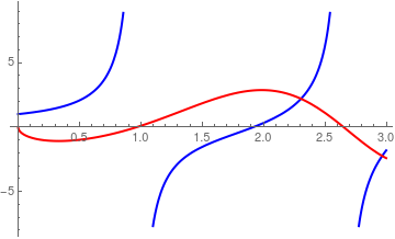
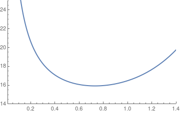
By plotting the denominator of Ricatti solution, we find approximately the point where its graph (in red) crosses the horizontal axis. This point indicates the position where the solution to the Riccati equation blows up. It is impossible to determine this point from the initial
value problem only. Fortunately, Mathematica can help with its determination.
FindRoot[deno[x], {x, 1}]
{x -> 0.969811}
Therefore, we know now that the solution (which is unique) to the given initial value problem exists only within the interval [0, 0.9698).
Our next step is to determine a power series representation for the solution.
We can find its 10-term Maclaurin series expansion with a one line Mathematica command:
At this point, although we know many terms in its Maclaurin series, it is impossible to find its radius of convergence because we don't know how coefficients grow.
According to G. Adomian, we seek the solution as an infinite sum
\[
y(x) = \sum_{n\ge 0} u_n ,
\]
where u0 is the unique solution of the following IVP:
\[
y' = x^2 , \qquad y(0) =1;
\]
which includes only the nonhomogeneous components of the original
IVP.
Using Mathematica, we obtain
Comparing the two-term Adomian approximation φ2(x) with the true Maclaurin expansion, we see that φ2(x) has correct first three terms and the noise terms:
This series reveals that the first terms up to the power 4 are correct.
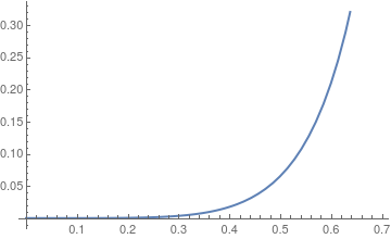
We next compare the last Adomian approximation with the true solution by calculating the error function.
Graph of the error function for Adomian four term approximation
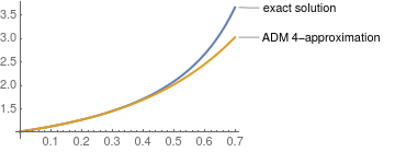
We compare our ADM approximation with true solution and approximation obtained with the aid of classical Runge--Kutta of order 4 (abbreviated by RK4) with step size h = 0.1.
Point
True value
ADM-4 approximation
RK4 approximation
x = 0.1
1.11146
1.11145
1.11146
x = 0.2
1.25302
1.25262
1.25302
x = 0.3
1.43967
1.43617
1.43967
Expantion of the true solution into the power series can be done directly:
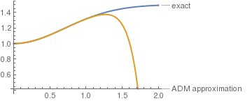
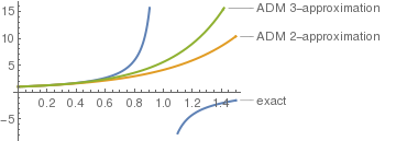
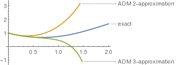
True solution and Adomian approximations with N=2 and 3 terms.
As we see from this graph, we can get a good approximation within a small interval [0,0.2]. To get a better approximation, however, we need to to add more terms. The solution has a singular point near x = 1, which we find by equating the denominator to zero in the explicit representation of the true solution:
Therefore, the true solution blows up around the point 0.969811, but
the power series approximation cannot detect the exact point no matter how
many terms we use.
Non standard ADM
We show how the ADM works when we split the initial condition between several few first Adomian components. So we choose the initial approximation as the solution of the following initial value problem:
Since all Adomian polynomails were determined previously, we find the next two components in the Adomian series by solving the following initial value problems:
We proceed in exactly the same way as in the previous example.
Now we are ready to determine the first five terms in the Adomian series by solving the recursive initial value problems:
True solution and Adomian approximations with N=2 and 3 terms.
As we see, the Adomian approximation with three terms ϕ3
matches the true solution up to power 3, and the rest are noise terms that contain x powers greater than 3. We eliminate some noise terms with the next iteration.
We compare our ADM approximations with the true solution and the approximation obtained with the aid of the classical Runge--Kutta of order 4 (abbreviated by RK4) with step size h = 0.1.
So we see that the 5-term ADM approximation is less accurate than the Runge--Kutta algorithm of order four; Also, the fomer requires more labor compared to the RK-4.
■
Example:
Consider the initial
value problem for the autonomous equation
According to the ADM, we assume that the solution can be represented by a convergent series
\[
y(x) = \sum_{n\ge 0} u_n (x) ,
\]
where the initial approximation is taken to be u0 = 3 because the given differential equation is autonomous. Substituting the infinite series into the given differential equation, we obtain
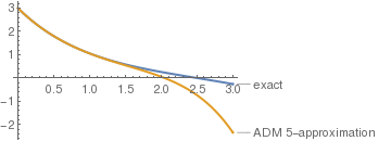
True solution and the Adomian approximation with N=5 terms.
■
Some modifications of the ADM
Since the ADM inverntion, many modifications and improvements
were introduced in its applications, including several algorithms for evaluation of Adomian's polynomials and their generalizations.
Instead of the standard ADM procedure, Abdul-Majid Wazwaz and some other researchers suggest splitting the inhomogeneous input between the first two (or more) terms in Adomian's series to minimize the influence of noise terms that are typical in nonhomogeneous equations. Another approach is based on splitting the initial condition between sequential initial value problems in order to increase the region of convergence for Adomian's decomposition solution. It represents the solution of the initial value problem
\[
y' = f(x,y) + g(x) , \qquad y(x_0 ) = y_0
\]
as the sum of components \( y(x) = u_0 + \sum_{n\ge 1} u_n (x) , \) where u0 and un, n ≥ 1, are solutions of the following initial value problems
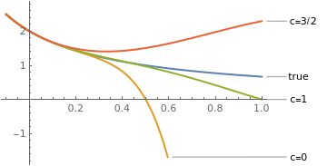
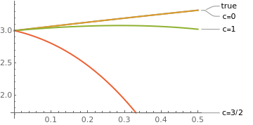
In order to see the effect of varying the value of c on the domain of convergence, we plot the curves of the explicit solution and fifth degree decomposition approximations for some values of c.
The Maclaurin series above for the true solution converges when |x| < 9/4 = 2.25. The coefficients of this power series are expressed through the binomial coefficients
True solution and 5-term approximations for some values of c.
■
G. Adomian, K. Malakian, A comparison of the iterative method and
Picard's successive approximations for deterministic and stochastic
differential equations, Applied Mathematics and Computation, Vol. 8,
No. 3, 187--204, 1981.
N. Bellomo, D. Sarafyan, On Adomian's decomposition method and some
comparisons with Picard's iterative scheme, Journal of Mathematical
Analysis and Applications, Vol. 123, No. 2, 389--400, 1987.
Duan, J.-S., Rach, R., Wang, Z., On the effective region of convergence of the decomposition series solution, Journal of Algorithms & Computational Technology, 2012, Vol. 7, No. 2, pp. 227--247.
Return to Mathematica page
Return to the main page (APMA0330)
Return to the Part 1 (Plotting)
Return to the Part 2 (First Order ODEs)
Return to the Part 3 (Numerical Methods)
Return to the Part 4 (Second and Higher Order ODEs)
Return to the Part 5 (Series and Recurrences)
Return to the Part 6 (Laplace Transform)
Return to the Part 7 (Boundary Value Problems)