Return to computing page for the first course APMA0330
Return to computing page for the second course APMA0340
Return to Mathematica tutorial for the second course APMA0340
Return to the main page for the course APMA0330
Return to the main page for the course APMA0340
Return to Part V of the course APMA0330
In what follows, we will use the summation notation, which not only reduces
the labor involved, but is often helpful in recognizing the general term of
the series. According to the notation, a series such as
\[
a_0 + a_1 + \cdots + a_n
\]
with a finite number of terms is represented by
\[
\sum_{j=0}^n a_j \qquad\mbox{or}\qquad \sum_{0\le j \le n} a_j
\qquad\mbox{or}\qquad \sum_{j \in [0..n]} a_j .
\]
The sign Σ is a Greek capital letter sigma, j is called
the summation index. Note that any letter or character can be used for the index j. The value j = 0 is referred to as the lower limit, while
j = n is referred to as the upper limit.
In the case where we have an infinite series
\[
a_0 + a_1 + \cdots + a_n + \cdots ,
\]
we represent it by
\[
\sum_{j=0}^\infty a_j \qquad\mbox{or}\qquad \sum_{j \ge 0} a_j .
\]
Infinite series are summations of infinitely many real or complex numbers or functions. They occur frequently in both pure and applied mathematics
as in accurate numerical approximations.
Infinite series are ubiquitous in the mathematical analysis
of scientific problems and numerical calculations because they appear in the evaluation of integrals, elementary and transcendental functions. The conventional approach for the evaluation of an infinite series consists in computing a finite sequence of partial sums
\[
s_n = \sum_{k=0}^n a_k
\]
by adding up one term after the other. If the sequence { sn }n≥0 of partial sums s0 = 𝑎0, s1 = 𝑎0 + 𝑎1, … , sn = 𝑎0 + 𝑎1 + ··· + 𝑎n converges, we say that the corresponding sum converges. If for convergent series, the partial sum is not obtained yet to the desired accuracy, additional terms must be added until convergence has finally been achieved. In principle, it is possible to determine the value of an infinite series as accurately as one likes provided that one is able to compute a sufficiently large number of terms accurately enough to overcome eventual numerical instabilities.
In practice, it is possible only to compute a relatively small number of terms. In addition, the series terms with higher summation indices are often affected by serious inaccuracies that may lead to a catastrophic accumulation of round-off errors. Consequently, if an infinite series is to be evaluated by adding one term after the other, an infinite series will be of practical use only if it converges after a sufficiently small number of terms.
In many practical problems involving differential equations, we come across infinite series with coefficients that depend on some parameter. For example, the ground state energy eigenvalue E(β) of the quartic anharmonic oscillator,
diverges for any real β. Therefore, some summation techniques have to be applied to give this Rayleigh--Schrödinger series any meaning beyond a mere formal expansion.
A power series in powers of x - x0 (or just power series) is an infinite
series of the form
where x0 is a fixed number, x is a variable, and the sequence
\( \displaystyle \left\{ c_n \right\}_{n\ge 0} \)
are often called the coefficients of the series.
The power series is said to converge to the function f(x) if
the sequence of partial sums
It turns out that we know more about convergence of power series.
For any power series
\( \displaystyle c_0 + c_1 (x-a) + c_2 (x-a)^2 + \cdots ,
\) in real variable x there is always a symmetric interval (𝑎-R, 𝑎+R) called the interval of convergence, in which a power
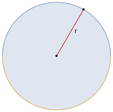
series converges, and diverges outside it. The number R is called the radius of convergence. If
x is complex, then the power series converges within a circle
\( |x-a| < R \) on complex plane ℂ.
Moreover, a power series always converges absolutely and uniformly within
its domain of convergence---a circle |x - 𝑎| < R. When the
radius of convergence is zero, we say that the power series diverges.
If the radius of convergence R = ∞, the sum-function
\( \displaystyle S(x) = \sum_{n\ge 0} c_n \left( x-a \right)^n \)
is called the
entire function.
Theorem: :
If a power series \( \sum_{n\ge 0} c_n \left( x-a \right)^n \) converges at x = x1 and diverges at x = x2, then the series converges absolutely for
\( | x- a | < | x_1 - a | \) and diverges for
\( | x- a | > | x_2 - a | . \)
There are known some tests for convergence of a power series. The following
two are the most popular.
Theorem: Root test:
The radius R of convergence for power series
\( \sum_{n\ge 0} c_n \left( x-a \right)^n \) is
the reciprocal to the limit superior (possibly ∞)
In formula \eqref{EqReview.3},
\( \overline{\lim} = \limsup_{n\to \infty} \) is the upper limit; correspondingly, \( \underline{\lim} = \liminf_{n\to \infty} \) is the lower limit.
A sequence
{ bk }k= p ∞ of real (or complex) numbers, bk, is said to
be a subsequence of the given sequence { 𝑎n } if there exists a
strictly increasing sequence { nk }k= p ∞ of integers such that
bk = 𝑎nk for every k ≥ p. The upper limit of the given sequence of
numbers { 𝑎n } is the largest limit of its any convergent subsequence.
For example, the sequence 𝑎n = (-1)n does not have a limit. However, for
even indices 𝑎2k =1 and for odd indices 𝑎2k+1 =-1. So, we have two
subsequences { 𝑎2k }k ≥ 0 and { 𝑎2k+1 }k ≥ 0 having
limits 1 and -1, respectively. Therefore, the upper limit of the sequence
(-1)n is 1, and its lower limit is just -1.
Theorem: Ratio test: (also known as D'Alembert's criterion).
Suppose that for a power series
\( \sum_{n\ge 0} c_n \left( x-a \right)^n ,\) there
there exists r such that
\begin{equation}
\lim_{n\to \infty} \left\vert \frac{c_{n+1}}{c_n} \right\vert = r.
\label{EqReview.4}
\end{equation}
The series is absolutely convergent when
\( \displaystyle \left\vert x-a \right\vert r < 1, \)
and diverges when \( \displaystyle \left\vert x-a
\right\vert r > 1. \) If \( \displaystyle \left\vert x-a \right\vert = 1/r, \) the ratio test is inconclusive, and the series may converge or not.
Other power series convergent tests are
collected in the following
web site.
Example:
Determine the interval of convergence for the power series
According to the D'Alembert's criterion, the series converges absolutely for
\( \displaystyle |x-1| < 1 , \) or
0 < x < 2, and diverges for
\( \displaystyle |x-1| > 1 . \)
The values of x corresponding to |x-1| = 1 are x = 0 and
x = 2. the power series diverges for each of these values of
x since the n-th term of the series does not approach zero as
n ↦ ∞.
■
We need to recall some definitions from the theory of functions of a complex variable that are related to power series.
A complex-valued function f(x) on a domain Ω ⊂ ℂ
is called holomorphic (or regular) if
at every point of its domain it is infinitely differentiable and equals, locally, to its own Taylor series:
where x0 is arbitrary point from the domain Ω of f.
The word derives from the Greek ολοσ (holos), meaning "whole," and μορφη (morphe), meaning "form" or "appearance." Maclaurin series is the special case when the center is zero: x0 = 0.
A complex-valued function is called analytic if its locally holomorphic at any point of its domain; it is obtained by analytic continuation by expanding the function into the corresponding Taylor series.
A complex function that is analytic at all finite points of the complex plane is said to be entire.
A holomorphic function is always a single-valued function meaning that for every input point from its domain, which is a subset of ℂ, the holomorphic function assigns a unique output (complex number). On the other hand, an analytic function maybe a multiple-valued function. For example, a square root function
\( f(z) = \sqrt{z} = z^{1/2} \) is an analytic function but not a holomorphic function on ℂ because it assigns two values to each input z ≠ 0. So \( \sqrt{-1} = \pm {\bf j} . \) Expanding the square root function into Taylor's series centered at 1, we obtain
\[
\sqrt{z} = 1 + \frac{1}{2}\left( z-1 \right) - \frac{1}{2^3} \left( z-1 \right)^2 +\frac{1}{2^4} \left( z-1 \right)^3 - \frac{5}{128} \left( z-1 \right)^4 + \frac{7}{256} \left( z-1 \right)^5 - \frac{21}{1024}\left( z-1 \right)^6 + \cdots ,
\]
Series[Sqrt[z], {z, 1, 10}]
which is the holomorphic function within a circle |z - 1| < 1.
Lazy people like me prefer to work with Maclaurin series because shifting
independent variable z = x - a reduces any Taylor's series to
its Maclaurin counterpart. For any holomorphic function f(z) in
a neighborhood of the origin, we can determine its power series (or
Maclaurin) coefficients according to the formula
An analytic function may consist of many holomorphic functions, called branches. From mathematical point of view, an analytic function may not be a function because its value at any point from the domain depends on what branch holomorphic function is used. Our objective is to use holomorphic functions to represent solutions to differential equations. Therefore, we will discuss only properties of holomorphic functions that will be used in our presentation of differential equations.
The first observation is that a holomorphic function is defined locally and it depends on derivatives evaluated at one point---the center of its Taylor series expansion. The infinitesimal knowledge of the function at one point (which is the center of Taylor's series) provides the complete information about the function within its interval of convergence because the function can be uniquely restored from its Taylor's coefficients. Obviously, Taylor's series is useless outside the interval of convergence unless you use another definition of convergence (which we will utilize in the second part of the tutorial). Taylor's series can be truncated to provide a polynomial approximation at points inside its interval of convergence:
The error En of such approximation is (in Lagrange form):
\[
f (x) = \sum_{k=0}^n \frac{f^{(k)} (a)}{k!} \left( x- a \right)^k + E_n (x) , \qquad\mbox{where} \quad E_n (x) = \frac{f^{(n+1)} (\xi )}{(n+1)!} \left( x- a \right)^{n-1},
\]
for some point ξ.
Example:
We use the function \( f(x) = e^{\cos 3x} , \)
and expand it into the
Maclaurin series around x=0.
The required approximation of the true value
1/e = 0.36787944117144232160
is obtained by using the truncated Maclaurin series with 10 terms
upon setting x=π:
Now we estimate the error on the interval [0,3] for the truncated Maclaurin
polynomial with n=10 degree polynomial. So we use Mathematica
and define
R[x_,c_] = x^(11) /11! D[f[y], {y,11}]/.y->c
Print["The Lagrange form of the remainder is"]
Print[""]
Print["R[x,c] = f^(11)[c]/11! x^(11) where c lies somewhere between 0 and x"]
Print[""]
Print["R[x,c] = ", Together[R[x,c]]]
First we need to bound the size of the term
\( \frac{f^{(11)} (c)}{11!} \)
for values of c in the interval 0 ≤ c ≤ 3.
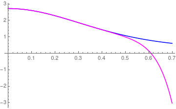
This can easily be done graphically, but to do it analytically with
derivatives is quite messy. We choose to look at the following graph to see
what is happening.
Approximation in magenta color and true function in blue
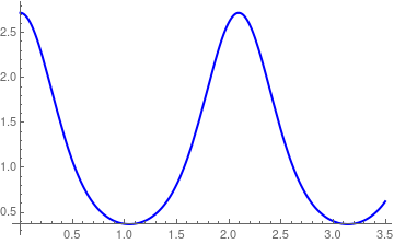
The graph of \( f(x) = e^{\cos 3x} \)
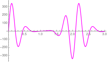
Error by 10-th degree polynomial approximation
How big does \( \frac{f^{(11)} (c)}{11!} \) get?
Looking at the graph we can estimate it does not exceed 350. However, Mathematica gives the exact answer:
FindMaximum[g[x], {x, 3}]
{341.589, {x -> 4.2888}}
One can find more accurate answer by using, for instance,
SetPrecision command.
■
If f(z) is analytic everywhere throughout some neighborhood of a point z = 𝑎, say inside a circle \( |z-a| = r , \) except at the point z = 𝑎 itself, then this point is called an
isolated singular point of f(z). The function
f(z) cannot be bounded near an isolated singular point.
An isolated singular point z = 𝑎 is called the pole if
f(z) is unbounded at z = 𝑎 and if in addition there exists
a positive integer n such that the product
\( \left( z- a \right)^n f(z) \) is holomorphic at
z = 𝑎.
An isolated singular point z = 𝑎 that is not a pole
(or removable singularity) is called an essential singularity.
When f(z) is a multi-valued analytic function, any point that
cannot be an interior point of the region of definition of a
single-valued branch (which is holomorphic) of f(z) is a singular branch point.
A typical example of multivalued analytic function gives either a square root
or logarithm.
Example:
Let us find Taylor's series expansion about x = 0 for the function
\( f(x) = e^{\cos 3x} , \) keeping terms to order
x11.
The above procedure of expanding a given function can be generalized using Mathematica. Here is a some force function f(x) that is expanded about x=0 to 5th order, given the name force.
Example:
Any polynomial is a holomorphic function in ℂ. For instance,
the polynomial f(x) = (x - 1)² is its Taylor expansion
centered at x = 1 because it contains only powers of x - 1:
\[
f(x) = 0 + 0\cdot (x-1) + (x-1)^2 + 0\cdot (x-1)^3 + \cdots .
\]
The Maclaurin series for the same function should contain only powers ofx,
so f(x) = 1 -2 x + x².
The Taylor series for f centered atx = 2 is
\[
f(x) = (x-2+1)^2 = \left[ (x-2) +1 \right]^2 = 1 + 2 (x-2) + (x-2)^2 .
\]
As we know, all these series expansions of f(x) = (x - 1)² are unique.
■
Now we list some useful properties of Taylor's series.
Addition and Subtraction.
Suppose that two series \( \displaystyle \sum_{n\ge 0} a_n
\left( x - x_0 \right)^n \quad\mbox{and} \quad \sum_{n\ge 0} b_n
\left( x - x_0 \right)^n \) converge to f(x) and
g(x),, respectively, for
\( \displaystyle \left\vert x - x_0 \right\vert < r, \
r > 0 . \) These two series can be added or subtracted termwise,
and
is called the convolution of the coefficients { 𝑎n }
and { bn }. The resulting series converges at least for
\( \displaystyle \left\vert x - x_0 \right\vert < r, \
r > 0 . \)
Division of Power Series.
If the holomorphic functions g(x) ≠ 0 in some neighborhood of x0, then the series \( f(x) = \sum_{n\ge 0} f_n \left( x- x_0 \right)^n \) for the sum-function of f(x) can be formally divided by the series for \( g(x) = \sum_{n\ge 0} g_n \left( x- x_0 \right)^n , \) and
Term-by-Term Differentiation.
The sum-function \( \displaystyle f(x) =
\sum_{n\ge 0} a_n \left( x- x_0 \right)^n \)
is continuous and has derivatives of all
orders for x from the interval of convergence
\( \displaystyle \left\vert x - x_0 \right\vert
< r, \ r > 0 . \) Moreover, its consecutive derivatives
f', f'', ... can be computed by differentiating the series termwise; that is,
and so forth, and each of the series converges absolutely for
\( \displaystyle \left\vert x - x_0 \right\vert
< r. \)
Uniqueness
If \( \displaystyle
\sum_{n\ge 0} a_n \left( x- x_0 \right)^n = \sum_{n\ge 0} b_n \left( x- x_0 \right)^n \) for each x in some open interval with center x0, then 𝑎n = bn for n = 0,1,2,3, ... . In particular, if \( \displaystyle
\sum_{n\ge 0} b_n \left( x- x_0 \right)^n = 0 \) for each such x, then b0 = b1 = ... = bn = ... = 0.
New Series by Substitution. In many cases, we can get new series from
old ones by substitution instead of applying Taylor series \eqref{E61.3},
because direct calculation of the derivatives may be more difficult and
cumbersome.
When a function is a product of two functions, finding its n-th
derivative can be obtained by a formula ascribed to Gottfried von
Leibniz (1646 -- 1712):
Example:
Let us find Maclaurin's expansion for \( f(x) \equiv \ln (ax+b)/(1-x), \quad b\ne 0. \) Since the required function is the product of two functions, we
apply the Leibniz formula \eqref{EqReview.6} to obtain
\[
f(x) = \sum_{n\ge 0} \frac{x^n}{n!} \, \left( D^n f \right) (0) =
\sum_{n\ge 0} \frac{x^n}{n!} \, \sum_{r=0}^n \binom{n}{r} \left( D^r
\ln (ax+b) \right) (0) \, \left( D^{n-r} \frac{1}{1-x} \right) (0) .
\]
So we need to find Maclaurin's coefficients of the logarithmic
function only because the second term, \( \texttt{D}^{n-r} \frac{1}{1-x} \,(0), \)
is known to be 1 for all derivatives. Using well-known formulas of the
derivatives of a power function
\[
\texttt{D}\,\frac{1}{ax+b} = -\frac{a}{(ax+b)^2} , \quad \texttt{D}^2 \frac{1}{ax+b} =
-\texttt{D}\,\frac{a}{(ax+b)^2} = \frac{2\,a^2}{(ax+b)^3}, \quad\mbox{and so on,}
\]
the derivatives of the logarithm can be calculated explicitly:
\[
\texttt{D}^r \ln (ax+b) = \texttt{D}^{r-1} \, \frac{a}{ax+b} = (-1)^{r-1} \,(r-1)! \,a^r
(ax+b)^{-r} , \qquad r\ge 1.
\]
Therefore,
\[
\ln (ax+b) =\ln b + \sum_{n\ge 1} (-1)^{n-1} \, \left( \frac{a}{b}
\right)^{n-1} \frac{x^n}{n}
\]
and taking convolution, we obtain
\begin{align*}
\frac{\ln (ax+b)}{1-x} &=\ln b +\left( \ln b + \frac{a}{b} \right) x +
\left( \ln b + \frac{a}{b} - \frac{a^2}{2b^2} \right) x^2 + \cdots \\
&= \ln b +\sum_{n\ge 1} \left( \ln b + \sum_{r=1}^n
(-1)^{r-1}\frac{a^r}{r\,b^r} \right) x^n .
\end{align*}
In the special case 𝑎 = b = 1, this reduces to the formula
\begin{align*}
\frac{\ln (1+x)}{1-x} &= \ln (1+x) (1 + x + x^2 + x^3 + \cdots ) \\
&=
\left( x-\frac{x^2}{2} + \frac{x^3}{3} -\frac{x^4}{4} + \cdots \right) (1 + x +
x^2 + x^3 + \cdots ) \\
&= x+\frac{1}{2}\,x^2 + x^3 \,\left( 1-\frac{1}{2} + \frac{1}{3} \right) +
x^4\,\left( 1-\frac{1}{2} + \frac{1}{3} -\frac{1}{4} \right) + \cdots \\
&= x + \frac{1}{2}\,x^2 + \frac{5}{6}\,x^3 + \frac{7}{12}\,x^4 +
\frac{47}{60}\,x^5 + \cdots .
\end{align*}
Another option to find the Maclaurin series is to multiply both sides
of the equation
\[
\frac{\ln (1+x)}{1-x} = \sum_{n=0}^\infty \,d_n\,x^n
\]
by (1-x) and set it equal to the resulting series. This yields
\begin{eqnarray*}
x-\frac{x^2}{2} + \frac{x^3}{3} -\frac{x^4}{4} + \cdots &=& (1-x)( d_0
+ d_1 x + d_2 x^2 + \cdots ) \\
&=& d_0 + ( d_1 - d_0 )x + ( d_2 - d_1 )\,x^2 + ( d_3 - d_2 )\,x^3 +
\cdots .
\end{eqnarray*}
Equating the like power terms, we obtain
\[
\begin{array}{ll}
d_0 =0 &\\
d_1 - d_0 =1 & d_1 =1\\
d_2 - d_1 = -\frac{1}{2} & d_2 = d_1 - \frac{1}{2} = \frac{1}{2} \\
d_3 - d_2 = \frac{1}{3} &d_3 = d_2 + \frac{1}{3} = \frac{5}{6}\\
d_4 - d_3 = -\frac{1}{4} & d_4 =d_3 -\frac{1}{4} = \frac{47}{60}\\
\cdots & \cdots \\
d_n - d_{n-1} = (-1)^{n-1} \,\frac{1}{n} & d_n = d_{n-1} + (-1)^{n-1}
\,\frac{1}{n} .\end{array}
\]
Solutions to the difference equation of the first order for dn are known as the derangement
numbers:
\[
d_n = 1 - \frac{1}{2} + \frac{1}{3} - \cdots + (-1)^{n-1} \,\frac{1}{n} .
\]
■
Example:
Suppose we want to find the Taylor series for \( \displaystyle f(x) =e^{x^2} \)
about x = 0, that is, in the form \( \displaystyle \sum_{n=0}^\infty \,a_n\,x^n . \) We
could find coefficients by direct differentiation to be
\[
a_n = \frac{f^{(n)} (0)}{n!} = \frac{1}{n!}\,\left. \frac{d^n}{dx^n} \left
( e^{x^2} \right)\right\vert_{x=0} .
\]
However, direct calculations by the chain rule will be tiresome. Fortunately,
there is a simpler way: substitute $y=x^2$ into the power series
\[
e^y = 1+y + \frac{y^2}{2!} + \frac{y^3}{3!} + \cdots + \frac{y^n}{n!} + \cdots
\quad \mbox{for all}\ y.
\]
This leads to
\[
e^{x^2} = 1 + x^2 + \frac{x^4}{2!} + \frac{x^6}{3!} +\cdots + \frac{x^{2n}}{n!}
+ \cdots \quad \mbox{for all}\ x.
\]
Let us find the Taylor series
about θ = 0 for f(θ) = esinθ.
We know the Taylor series of ey and sinθ to be
\[
e^y = 1 + y + \frac{y^2}{2!} + \frac{y^3}{3!} +\cdots = \sum_{n=0}^\infty
\,\frac{y^n}{n!}
\]
and
\[
\sin\theta = \theta - \frac{\theta^3}{3!} + \frac{\theta^5}{5!} - \cdots
=\sum_{k=0}^\infty\, (-1)^k \,\frac{\theta^{2k+1}}{(2k+1)!} .
\]
Let us substitute the series for sinθ for y. This yields
\begin{align*}
e^{\sin \theta} &= 1 + \left( \theta - \frac{\theta^3}{3!} + \frac{\theta^5}{5!}
- \cdots \right)
\\
&\quad +
\frac{1}{2!}\,\left( \theta - \frac{\theta^3}{3!} + \frac{\theta^5}{5!} -
\cdots \right)^2 + \frac{1}{3!}\,\left( \theta - \frac{\theta^3}{3!} +
\frac{\theta^5}{5!} - \cdots \right)^3 + \cdots
\end{align*}
Collecting similar terms, we obtain
\begin{eqnarray*}
e^{\sin \theta}&=&1 + \theta +\frac{\theta^2}{2!} +\left( -\frac{\theta^3}{3!}
+ \frac{\theta^3}{3!} \right) + \left( \frac{\theta^4}{4!} -
\frac{\theta^4}{3!} \right) + \cdots
\\
&=& 1 + \theta +\frac{\theta^2}{2!} - \frac{2}{4!}\,\theta^4 +
\cdots \quad \mbox{for all}\ \theta .
\end{eqnarray*}
■
Shifting indices in a power series
The index of summation in any series is a dummy parameter just as in the integration variable in a definite integral is a dummy variable. Hence, it is immaterial which letter is used for the index of summation. For example
Just as we make changes of the variable of integration in a definite integral, we find it convenient to make changes of summation indices in calculating series solutions of differential equations. As we differentiate sum-function, we
obtain a series with shifted indices in its coefficients.
The process of shifting (or slipping) indices can be obtained by the following Mathematica code:
SlipIndices[Op_[expr_, {k_, a_, b_}], d_] :=
Op[(expr /. k -> k + d), {k, a - d, b - d}] \
As an example, consider shifting indices in the sum:
It is frequently necessary to compare the magnitude of two functions or sequences. For example, it is clear that, for large enough n,
𝑎n = 2 + n³ is larger than bn = n·101000 and smaller than cn = n3.5, but how can we conveniently express this idea?
Therefore, we introduce the following order symbols.
Let f(z) and g(z) be two functions defined on some domain Ω in the complex plane ℂ and let z0 be a limit point of Ω, possibly the point at infinity. Then,
\[
f(z) = O \left( g(z) \right)
\]
means that there is a positive constant K and a neighborhood U ∋ z0 such that
\[
\left\vert f(z) \right\vert \le K \left\vert g(z) \right\vert
\]
for all z ∈ U∩Ω. If g(z) does not vanish on U∩Ω, this simply means that the ratio f(z)/g(z) is bounded on U∩Ω. Also,
\[
f(z) = o \left( g(z) \right)
\]
means that for any positive number ϵ there exists a neighborhood U of z0 such that
for all z ∈ U∩Ω. If g(z) does not vanish on U∩Ω, this simply means that the ratio f(z)/g(z) approaches zero when z ↦ z0.
Dettman, J.W., The solution of a second order linear differential equation near a regular singular point,
The American Mathematical Monthly, 1964, Vol. 71, No. 8, pp. 378--385.
https://doi.org/10.1080/00029890.1964.1199225
Dettman, J.W., Power Series Solutions of Ordinary Differential Equations, The American Mathematical Monthly, 1967, Vol. 74, No. 4, pp. 428--430. https://doi.org/10.2307/2314582
Grigorieva, E., Methods of Solving Sequence and Series Problems, Birkhäuser; 1st ed. 2016.
Return to Mathematica page
Return to the main page (APMA0330)
Return to the Part 1 (Plotting)
Return to the Part 2 (First Order ODEs)
Return to the Part 3 (Numerical Methods)
Return to the Part 4 (Second and Higher Order ODEs)
Return to the Part 5 (Series and Recurrences)
Return to the Part 6 (Laplace Transform)
Return to the Part 7 (Boundary Value Problems)