Preface


We discuss some classes of differential equations that can be reduced to a separable one with an appropriate substitution.

Return to computing page for the first course APMA0330
Return to computing page for the second course APMA0340
Return to Mathematica tutorial for the second course APMA0340
Return to the main page for the course APMA0330
Return to the main page for the course APMA0340
Return to Part II of the course APMA0330

Equations Reducible to Separable Equations


Changing variables


Sometimes it is convenient to interchange dependent and independent variables. There are cases when the given differential equation \( \frac{{\text d}y}{{\text d}x} = f(x,y) \) is very hard or impossible to solve while the inverse equation \( \frac{{\text d}x}{{\text d}y} = \frac{1}{f(x,y)} \) can be relatively easily handled. In this case, we consider x = x(y) as a function of y.

Example: Consider the initial value problem

\[ y' = \left( 2x-3y+5 \right)^{-1} , \qquad y(0) = 1. \]
To find its solution, we use standard Mathematica command

ans1 = DSolve[{y'[x] == 1/(2*x - 3*y[x] + 5), y[0] == 1}, y[x], x]
Out[1]= {{y[x] -> 1/6 (7 + 4 x - 3 ProductLog[1/3 E^(1/3 + (4x)/3)])}}
Plot[y[x] /. ans1, {x, -1, 1}, PlotRange -> {0.4, 1.5}, AspectRatio -> 1]
StreamPlot[{1, 1/(2*x - 3*y + 5)}, {x, -3, 3}, {y, -2, 3},
StreamPoints -> {{{{0, 1}, Red}, Automatic}}, StreamStyle -> Blue,
Background -> LightGray]
   
So Mathematica provides a solution expressed through a special function. Therefore, we try another approach based on the inverse problem when x is considered to be a dependent variable:
\[ \frac{{\text d}x}{{\text d}y} = \left( 2x-3y+5 \right) , \qquad x(1) = 0. \]
Since the equation is linear, we can find its solution without a problem.
ans2 = DSolve[{x'[y] == 2*x[y] - 3*y + 5, x[1] == 0}, x[y], y] // Simplify
Out[3]= {{x[y] -> 1/4 (-7 + E^(-2 + 2 y) + 6 y)}}
Plot[x[y] /. ans2, {y, 0.4, 1.5}, PlotRange -> {-1, 1}, AspectRatio -> 1]

Here is a way to flip the above graph:
ParametricPlot[Evaluate[{x[y], y} /. ans2], {y, 0, 2}, PlotRange -> {{-1, 1}, {0.4, 1.5}}, AspectRatio -> 1]


Linear Substitution


We present several classes of equations that can be reduced to a separable one. We start with the differential equation of the form

\begin{equation} y' = F(ax +by +c), \qquad b\ne 0, \label{EqReduce.1} \end{equation}
where F(v) is a given continuous function of a variable v, and a,b,c are some constants. This equation is reduced to a separable one by substitution \( v=ax+by +c . \)

Example: Consider the differential equation

\[ y' = 2x+3y+5 , \]
Using substitution v = 2x+3y+5, we find its derivative to be v' = 2 +3 y' = 2 + 3 v, which is a separable one. Separating variables and integrating, we obtain

\[ \frac{{\text d}v}{2+3v} = {\text d}x \qquad \Longrightarrow \qquad \ln \left( 2+ 3v \right) = 3x+C , \]
where C is an arbitrary constant. Exponentiation yields the general solution in implicit form:
\[ 2+3v = C\,e^{3x} \qquad \Longrightarrow \qquad 2+ 3\left( 2x+3y +5 \right) = C\,e^{3x} . \qquad ■ \]

Another class of equations is

\begin{equation} x\,y' = y\,F(xy), \label{EqReduce.2} \end{equation}

where F(v) is a function of the product v=xy. This differential equation is reduced to a separable one by substitution v=xy.

Example: First, we find solutions to the equation \( xy'=x^2 y^3 -y \) using the standard Mathematica command:

DSolve[y'[x] == x*(y[x])^3 -y[x]/x,y[x],x]
and then plot corresponding family of solutions:
solution = DSolve[y'[x] == x*(y[x])^3 - y[x]/x, y[x], x]
g[x_] = y[x] /. solution[[1]]
t[x_] = Table[g[x] /. C[1] -> j, {j, 1, 6}]
Plot[t[x], {x, 0.2, 3}]


Next we find its solution manually; we set v=xy, and get
\[ v' = y + x\,y' = y + x^2 y^3 -y = x^2 \left( \frac{v}{x} \right)^3 = \frac{v^3}{x} , \]
which is a separable one. So we separate variables and integrate
\[ \frac{{\text d}v}{v^3} = \frac{{\text d}x}{x} \qquad \Longrightarrow \qquad - \frac{1}{v^2} = 2\,\ln Cx = \ln C\,x^2 , \]
where C is an arbitrary positive constant. Upon returning for original dependent variable v=xy, we get the general solution in implicit form:
\[ \frac{1}{y^2} = -x^2 \ln C\,x^2 \qquad \mbox{or} \qquad 1 + x^2 y^2 \,\ln C x^2 =0. \]


Equations with Homogeneous Slope Function


Let r be a real number. A function of two variables g(x,y) is called homogeneous of degree r if \( g( \lambda x, \lambda y ) = \lambda^r g(x,y) \) for any nonzero constant λ. Usually homogeneous functions of zero degree are referred to as homogeneous or homogeneous-polar (because the ratio y/x in polar coordinates is the tangent of the angle). Obviously, a function of the ratio y/x is a homogeneous-polar function.

Our next class includes differential equations with homogeneous coefficients when the slope function is a function depending on the ratio y/x:

\begin{equation} y' = F(y/x) . \label{EqReduce.3} \end{equation}
This equation is reduced to a separable one by substitution v(x) = y/x or y=xv. Indeed, applying the product rule, we find
\[ \frac{{\text d}y}{{\text d}x} = \dfrac{\text d}{{\text d}x} \left( x\,v \right) = x\,\frac{{\text d}v}{{\text d}x} + v = x\, v + v . \]
Upon substituting this expression into the equation \( y' = F(y/x) = F(v) , \) we get
\[ x\,\frac{{\text d}v}{{\text d}x} + v = F( v) \qquad \mbox{or} \qquad x\, v' = F(v) -v . \]
The latter is a separable equation, which upon separation of variables and integration yields
\[ \int \frac{{\text d}v}{F(v) -v} = \int \frac{{\text d}x}{x} = \ln Cx , \qquad F(v) \ne v \qquad\mbox{and} \qquad v = y/x , \]
where C is an arbitrary constant (positive when x positive and negative when x is negative).

One particular important class of differential equations constitute the equations with linear coefficients:

\[ \left( Ax + By \right) {\text d}y = \left(ax+by \right) {\text d}x \qquad \mbox{or} \qquad \frac{{\text d}y}{{\text d}x} = \dfrac{ax+by}{Ax+By} = \dfrac{a+by/x}{A+By/x} , \]
where a, b, A, and B are known real constants. Upon substitution v = y/x, the above equation is reduced to a separable one:
\[ x\, \frac{{\text d}v}{{\text d}x} = \dfrac{a+bv - Av - B v^2}{A+Bv} \qquad \Longrightarrow \qquad \int \frac{A + Bv}{a + b(b-A) - B v^2}\, {\text d}v = \int \frac{{\text d}x}{x} = \ln Cx , \]
with some arbitrary constant C. The value of the integral over v depends on whether the roots of quadratic equation \( Bv^2 + (A-b) \,v - a =0 \) are distinct real, complex conjugate, or one double root.

Example: We consider the differential equation with homogeneous slope function

\[ y' = \frac{y-x}{y+x} = \dfrac{y/x -1}{y/x +1} . \]
Changing the dependent variable to v=y/x or \( y(x) = x\,v(x) , \) we obtain a separable equation in variable v:
\[ y' = v(x) + x\,v' (x) = \frac{v-1}{v+1} \qquad\Longrightarrow \qquad x\,v' = \frac{v-1}{v+1} -v = - \frac{v^2 +1}{v+1} . \]
Separation of variables yields
\[ \frac{v+1}{v^2 +1}\,{\text d}v = - \frac{{\text d}x}{x} \qquad\Longrightarrow \qquad \arctan v + \frac{1}{2}\,\ln (v^2 +1 ) = \int \frac{v+1}{v^2 +1}\,{\text d}v = - \int \frac{{\text d}x}{x} = -\ln Cx . \]
points := Tuples[{-2, -1, 0, 1, 2}, 2]
Table[StreamPlot[{1, {(y - x)/(x + y)}}, {x, -3, 3}, {y, -3, 3},
StreamPoints -> {points, Automatic, maxlen}, Epilog -> Point[points]],
{maxlen, {2.5, Scaled[.05]}}]
   

Example: Consider the differential equation

\[ \left( 9x -y \right) {\text d}x + \left( 7x+y \right) {\text d}y =0 \qquad 7x+y \ne 0. \]
Substitution v = y/x yields
\[ v + x\, v' = \frac{v-9}{v+7} \qquad\Longrightarrow \qquad \frac{\left( v+7 \right) {\text d}v}{v^2 + 6v +9} = -\frac{{\text d}x}{x} . \]
Integrating both sides, we get the general solution in implicit form:
\[ \frac{4}{v+3} + \ln x \left( v+3 \right) = C \qquad\Longrightarrow \qquad \frac{4x}{3x+y} + \ln \left\vert y + 3x \right\vert = C , \]
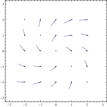
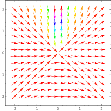
which is the general solution. Of course, we have to exclude the singular solution y = -3x 
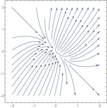
from the implicit formula. Finally, we plot the direction fields using VectorPlot command:
VectorPlot[{1, (y - 9*x)/(7*x + y)}, {x, -1, 1}, {y, -1, 1},
VectorPoints -> Fine, StreamPoints -> Coarse, StreamStyle -> Red, StreamScale -> Full]
points = Join[{#, -1.} & /@ Range[-1, 1, .2], {#, 1.} & /@ Range[-1, 1, .2]];
VectorPlot[{1, (y - 9*x)/(7*x + y)}, {x, -1, 1}, {y, -1, 1},
VectorPoints -> Fine, StreamPoints -> {points, Automatic, 2},
StreamStyle -> Orange, StreamScale -> Large]
Manipulate[points = Table[{Cos@t, Sin@t}*r, {t, 0., 2. \[Pi], d}];
VectorPlot[{1, (y - 9*x)/(7*x + y)}, {x, -1, 1}, {y, -1, 1},
VectorPoints -> Fine, StreamPoints -> {points, Automatic, l},
StreamStyle -> Blue, StreamScale -> Large,
Epilog -> {Green, PointSize@Large, Point@points}], {{d, \[Pi]/20., "point spacing"}, 0, 1, \[Pi]/40,
Appearance -> "Labeled"}, {{l, 2, "stream length"}, 0, 2,
Appearance -> "Labeled"}, {{r, 1, "radius"}, 0, 1, Appearance -> "Labeled"}]
     

Example: Consider the differential equation

\[ \frac{{\text d}y}{{\text d}x} = \frac{2x+4y}{3x+y} \qquad 3x\ne y . \]
Introducing a new dependent variable v = y/x, we reduce our differential equation to a separable one:
\[ v + x\, v' = \frac{2+4v}{v+3} \qquad\Longrightarrow \qquad \frac{\left( v+3 \right) {\text d}v}{v^2 - v -2} = -\frac{{\text d}x}{x} , \quad v \ne 2, \quad v\ne -1. \]
Since \( \frac{\left( v+3 \right) {\text d}v}{v^2 - v -2} = \frac{5/3}{v-2} - \frac{2/3}{v+1} , \) we integrate to obtain the general solution
\[ \frac{5}{3}\, \ln |v-2| - \ln \left\vert v+1 \right\vert = -C\, \ln |x| \qquad\Longrightarrow \qquad \frac{|v-2|^5}{(v+1)^2} = C\, |x|^{-3} . \]
Upon returning to the original variable y = xv, we get the general solution in implicit form:
\[ |y-2x|^5 = C\,(y+x)^2 \qquad (C \mbox{ is a constant}). \]
Initially, we excluded two solutions y = 2x and y = -x from our derivation because they appeared under the logarithm sign. Now we see that they could be obtained from the general solution and, therefore, are not singular solutions. 
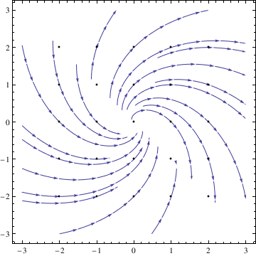
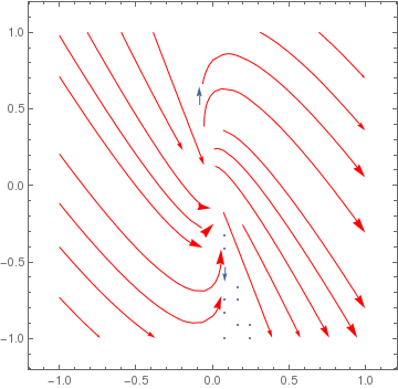
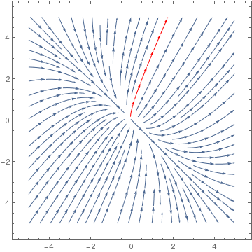
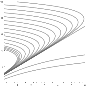
We plot direction fields with StreamPlot command. First, we just use the regular approach by identifying points and then apply the main command:
points = With[{d = .1}, Join[#, -#] &[{#, -2 + d} & /@ DeleteCases[Range[-2, 2, 1/5], x_ /; Not[FreeQ[x, -2 | 0 | 2]]]]];
Semicolumn suppresses output to be visible on the screen. We use the set of points in the next command to plot solutions through these points.
StreamPlot[{1, (2*x + 4*y)/(3*x + y)}, {x, -2, 2}, {y, -2, 2},
StreamPoints -> {points, Automatic}, StreamScale -> {{0.4, 0.01},(*or use Full to completely prevent segmentation*)All, 0.02, Automatic}]
However, Mathematica allows us to identify a point on this plot and then draw a particular trajectory through this point:
StreamPlot[{1, (2*x + 4*y)/(3*x + y)}, {x, -5, 5}, {y, -5, 5}, StreamPoints -> {{{{0.5, 2}, Red}, Automatic}}]
sp = StreamPlot[{1, (2*x + 4*y)/(3*x + y)}, {x, -5, 5}, {y, -5, 5}, StreamPoints -> {{{{0, 2}, White}, Automatic}},
Epilog -> {Red, PointSize[Large], Point[{0.5, 2}]}]
sp2 = StreamPlot[{1, (2*x + 4*y)/(3*x + y)}, {x, -5, 5}, {y, -5, 5},
StreamPoints -> {{{{0.5, 2}, Red}}}, RegionFunction -> (# > 0 &)]
Finally, we unite two previous pictures into one:
Show[sp, sp2]
     

Example: We demonstrate reduction of the equation with homogeneous slope function, y' =-(x^2 + y^2)/(5xy), to a separable equation. Of course, Mathematica is an appropriate tool for such reduction. We start with defining the differential equation with differentials.

ode[x_, y_] = -(x^2 + y^2)*dx == 5*x*y*dy
Out[8] = dx (-x^2 - y^2) == 5 dy x y
The first step is to replace the differential dy with the sum dy=xdv + vdx according to the product rule.
ode[x, v*x] /. {dy -> x*dv + v*dx}
Out[9] = dx (-x^2 - v^2 x^2) == 5 v x^2 (dx v + dv x)
Then we substitute instead of y the product y=xv:
Map[Cancel, Map[Function[q, q/x^2], %]]
Out[10] = -dx (1 + v^2) == 5 v (dx v + dv x)
Finally, we simplify the output by collecting similar terms.
Map[Function[u, Collect[u, {dx, dv}]], %]
Out[11] = -dx (1 + v^2) == 5 dx v^2 + 5 dv v x

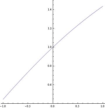
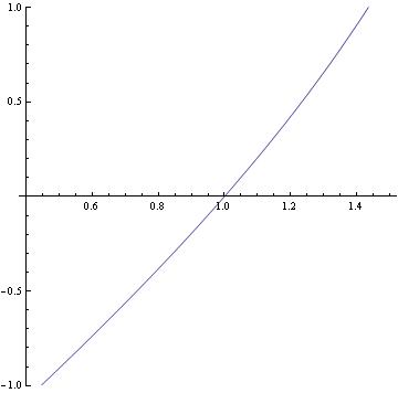
Example: : Consider the initial value problem y' = 1/(x-y+2),       y(0) =1 .

We find its solution and plot it using the following Mathematica commands:

ans1 = DSolve[{y'[x] == 1/(x - y[x] + 2), y[0] == 1}, y[x], x]
Plot[y[x] /. ans1, {x, -1, 1}, PlotRange -> {0, 2}, AspectRatio ->1]
ans2 = DSolve[{x'[y] == x[y] - y + 2, x[1] == 0}, x[y], y] //Simplify
ParametricPlot[Evaluate[{x[y], y} /. ans2], {y, 0, 2},
PlotRange -> {{-1, 1}, {0, 2}}, AspectRatio -> 1]

LineIntegralConvolutionPlot[{{1, 1/(x - y + 2)},
Image[Table[((-1)^i (-1)^j + 1)/2, {i, 45}, {j, 45}]]}, {x, -3,
3}, {y, -3, 3}, LineIntegralConvolutionScale -> 2,
ColorFunction -> GrayLevel, RasterSize -> 300]
StreamPlot[{1, 1/(x - y + 2)}, {x, -3, 3}, {y, -3, 3}, StreamStyle -> "Drop"]
   
We can plot solutions more clearly:
f = Solve[x == ans2[[1, 1, 2]], C[1]]
contourval = Table[(f[[1, 1, 2]]) /. {x -> 1, y -> i}, {i, 1, 10, 1/2}]
cp1 = ContourPlot[f[[1, 1, 2]], {x, 0.01, 6}, {y, 0, 10},
PlotPoints -> 150, Frame -> False, Contours -> contourval,
Axes -> Automatic, AxesOrigin -> {0, 0},
ContourStyle -> {{GrayLevel[0.4], Thickness[0.01]}},
ContourShading -> False, DisplayFunction -> Identity]

Example: : Suppose that an airplane is positioned at point B(2000,0) to fly to another airport O(0,0) that is 2000 km directly west of its position B. Assume that the airplane aims towards O at all times. If the wind goes from south to north at a constant speed w, and the airplane's speed in still air is v (which is greater than w), determine the airplane's path.

Observe that the derivative \( {\text d}y/{\text d}x \) describes the airplane's velocity in the x direction:

\[ \frac{{\text d}y}{{\text d}x} = -v\,\sin \theta + w = \frac{vx}{\sqrt{x^2 + y^2}} +w , \]
so
\[ \frac{{\text d}y}{{\text d}x} = \frac{{\text d}y / {\text d}t}{{\text d}x / {\text d}t} = \dfrac{ \frac{-vy}{\sqrt{x^2 + y^2}} +w}{\frac{-vx}{\sqrt{x^2 + y^2}}} = \frac{vy - w\sqrt{x^2 + y^2}}{vx} . \]
This is an equation with homogeneous slope function that could be written as
\[ \frac{{\text d}y}{{\text d}x} = \frac{y}{x} - \frac{w}{v}\,\sqrt{1 + \left( \frac{y}{x} \right)^2} . \]
Therefore, we must solve the initial value problem
\[ \frac{{\text d}y}{{\text d}x} = \frac{vy - w\sqrt{x^2 + y^2}}{vx} , \qquad y(2000) =0. \]
This equation we solve with the aid of Mathematica:
DSolve[{y'[x] == (v*y[x] - w*Sqrt[x^2 + y[x]^2])/v/x }, y[x], x]
{{y[x] -> x Sinh[(v C[1] - w Log[x])/v]}}
Obviously, C[1] = (w/v Log[2000] gives the required solution to the initial value problem.     ■
Example: Consider the differential equation
\[ \frac{{\text d}y}{{\text d}x} = \frac{y+ \sqrt{y^2 -x^2}}{x} \qquad\mbox{or} \qquad y = x\,y' - \sqrt{y^2 -x^2} , \qquad x \ne 0. \]
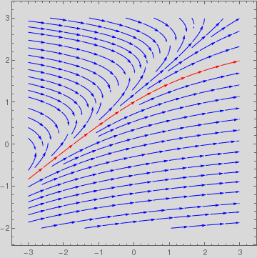
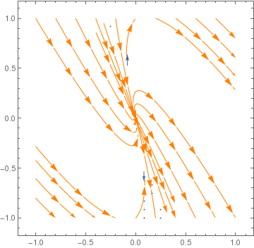
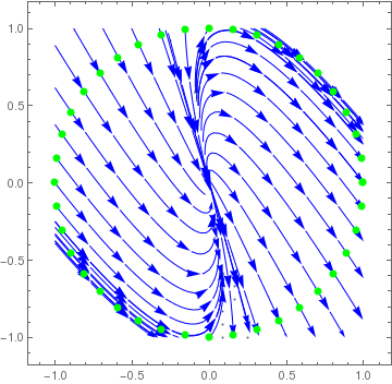
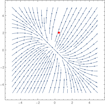
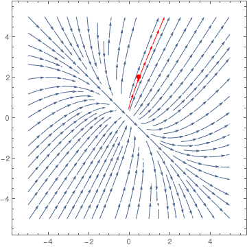
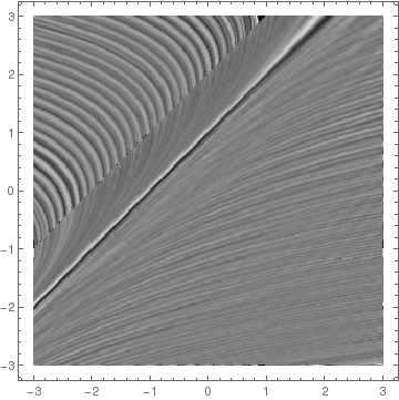
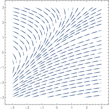
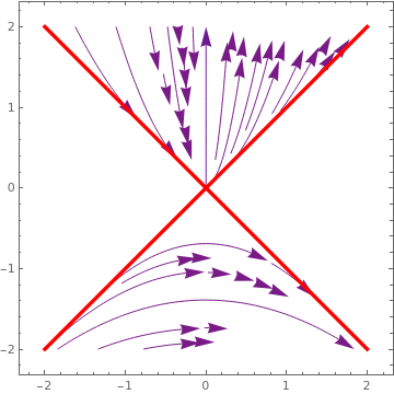
First, we plot direction field using VectorPlot command and then StreamPlot. Since the slope function is defined only for yx, we see that the former does not provide an adequate qualitative information.
VectorPlot[{1, y/x + Sqrt[y^2 - x^2]/x}, {x, -2, 2}, {y, -2, 2}, VectorScale -> {Small, Automatic, None}, VectorColorFunction -> Hue, VectorPoints -> 14]
field = StreamPlot[{1, y/x + Sqrt[y^2 - x^2]/x}, {x, -2, 2}, {y, -2, 2}, StreamColorFunction -> "Rainbow", StreamPoints -> 40, StreamScale -> {Full, All, 0.04}];
line1 = Graphics[{Red, Thickness[0.01], Line[{{-2, -2}, {2, 2}}]}];
line2 = Graphics[{Red, Thickness[0.01], Line[{{-2, 2}, {2, -2}}]}];
Show[field, line1, line2]
     
       Direction field plotted with VectorPlot.            ;Direction field plotted with StreamPlot.

Since x = 0 is a singular point, we exclude it from our consideration. Also the slope function is defined only for yx, we have to solve the given differential equation in the domain
\[ \Omega = \left\{ (x,y) \in \mathbb{R}^2 : \ |y| \ge |x| \quad\mbox{and} \quad x \ne 0 \right\} . \]
Making substitution y = x·v, we reduce the given differential equation to a separable one:
\[ x\,\frac{{\text d}v}{{\text d}x} + v = v + \sqrt{v^2 -1} \qquad\mbox{or} \qquad x\,\frac{{\text d}v}{{\text d}x} = \sqrt{v^2 -1} . \]
Separation of variables and integration yields
\[ x\,\frac{{\text d}v}{\sqrt{v^2 -1}} = \frac{{\text d}x}{x} \qquad \Longrightarrow \qquad \ln \frac{\sqrt{v^2 -1} +v}{\sqrt{v^2 -1} -v} = 2\,\ln |x| + \ln C \]
Upon exponentiation, we get the general solution
Integrate[1/Sqrt[v^2 - 1], v]
-(1/2) Log[1 - v/Sqrt[-1 + v^2]] + 1/2 Log[1 + v/Sqrt[-1 + v^2]]
\[ \frac{\sqrt{v^2 -1} +v}{\sqrt{v^2 -1} -v} = C\,x^2 , \qquad v^2 > 1, \quad x \ne 0, \]
where C is a not negative constant. The differential equation for v has two singular solutions v = ±1. Correspondingly, the given differential equation has the general solution
\[ \frac{\sqrt{y^2 -x^2} +y}{\sqrt{y^2 -x^2} -y} = C\,x^2 , \qquad y^2 > x^2 , \quad x \ne 0, \]
and two singular solutions that are marked in red in the figure above.    ■


Return to Mathematica page)
Return to the main page (APMA0330)
Return to the Part 1 (Plotting)
Return to the Part 2 (First Order ODEs)
Return to the Part 3 (Numerical Methods)
Return to the Part 4 (Second and Higher Order ODEs)
Return to the Part 5 (Series and Recurrences)
Return to the Part 6 (Laplace Transform)
Return to the Part 7 (Boundary Value Problems)