Preface
This section gives an introduction to a particular class of iterative root finding methods, called open methods. As opposed to closed or bracketing methods (discussed in the previous section), open methods do not necessarily bracket a root; therefore, they may diverge as computation progresses, but when they do converge, open methods are usually so much faster than bracketing methods. The root finding methods are applied for solving nonlinear equations of the form f(x) = 0. These are the problems of applied mathematics that occur most often for which explicit solutions are not available. We present some iterative algorithms for the determination of roots of these equations to any specified degree of accuracy. There are two large classes of iterative numerical methods for root finding, namely those that either involve a usage of derivatives or not.
We begin with Newton's method and its discretization---the secant method, which provide root-finding algorithms that use a succession of roots of secant lines to better approximate a root of a function f. The secant method can be thought of as a finite-difference approximation of Newton's method. The section also contains some iterative algorithms to find a root of a nonlinear equation f(x) = 0 of order two and larger.
Return to computing page for the second course APMA0340
Return to computing page for the fourth course APMA0360
Return to Mathematica tutorial for the first course APMA0330
Return to Mathematica tutorial for the second course APMA0340
Return to Mathematica tutorial for the fourth course APMA0360
Return to the main page for the course APMA0330
Return to Part III of the course APMA0330 Return to the main page for the course APMA0340
Return to the main page for the course APMA0360
Glossary
Example 1: Let \( f(x) = x^5 -5x+3 \) and we try to find its null, so we need to solve the equation \( x^5 -5x+3 =0 . \) Mathematica provides two real positive roots:
Let us add and subtract x from the equation: \( x^5 -5x+3+x =x . \) Expressing x, we derive another fixed point formula
I. Newton’s Method or Newton--Raphson Method
|
\[
x_{k+1} = x_k - \frac{f(x_k)}{f' (x_k )} , \qquad k=0,1,2,\ldots .
\tag{Newton.1}
\]
|
|---|
A concept of the the algorithm (Newton.1) was introduced by Isaac Newton in 1669, who used it to solve a cubic equation numerically. Before Newton other people also suggested analogous methods. The essential ideas of the method can be found in manuscripts of the fourteenth century written by the Persian astronomer and mathematician Ghiyāth al-Kāshī (1380--1429). His method of root-finding was not known by his contemporary mathematicians. We know that the English mathematician Henry Briggs (1561--1630) also published a work involving the numerical solution of polynomial equation in 1633. In 1685, John Wallis (1616--1703) described a method which---Willis said---was invented by I.Newton. However, the first systematic description of the method was given by J.Raphson in Aequationum Universalis, seu Ad Aequationes Algebraicas Resolvendas Methodus Generalis, & Expedita, Ex Nova Infinitarum Serierum Methodo, Deducta et Demonstrata (London, 1690).
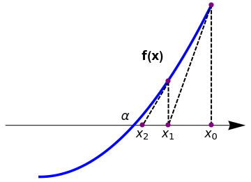
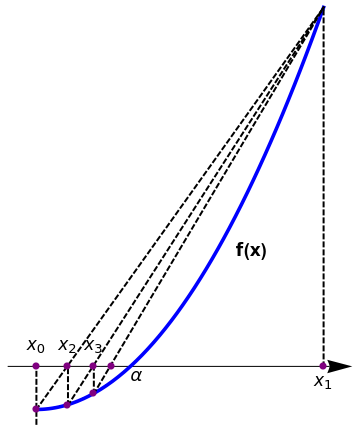
The basic idea behind Newton's method is quite straightforward. Let xn denote the most recent approximation to zero, α, of the function f. Replace f by its tangent line approximation that goes through the point xn and takes the x-intercept of the tangent line as the next approximation xn+1 to the root.
|
plot = Plot[1*x^2, {x, 0, 1}, AspectRatio -> 1,
PlotStyle -> {Thickness[0.01], Blue}, Axes -> False,
Epilog -> {PointSize[0.03], Pink, Point[{{0, 0}, {2, 2.8}}]},
PlotRange -> {{-0.5, 1.2}, {-0.2, 1.4}}];
arrow = Graphics[{Arrowheads[0.07], Arrow[{{-0.2, 0.3}, {1.2, 0.3}}]}]; l1 = Graphics[{Thick, Dashed, Line[{{1, 1}, {0.75, 0.3}}]}]; l2 = Graphics[{Thick, Dashed, Line[{{0.75, 0.55}, {0.6, 0.3}}]}]; l3 = Graphics[{Thick, Dashed, Line[{{1, 1}, {1, 0.3}}]}]; l4 = Graphics[{Thick, Dashed, Line[{{0.75, 0.55}, {0.75, 0.3}}]}]; t2 = Graphics[{Black, Text[Style[Subscript[x, 0], 16], {1, 0.25}]}]; t3 = Graphics[{Black, Text[Style[Subscript[x, 1], 16], {0.75, 0.25}]}]; t4 = Graphics[{Black, Text[Style[Subscript[x, 2], 16], {0.6, 0.25}]}]; t5 = Graphics[{Black, Text[Style[\[Alpha], 16], {0.5, 0.35}]}]; t9 = Graphics[{Black, Text[Style["f(x)", Bold, 16], {0.66, 0.7}]}]; Show[arrow, plot, l1, l2, l3, l4, t2, t3, t4, t5, t9, Epilog -> {PointSize[0.02], Purple, Point[{{0.6, 0.3}, {0.75, 0.555}, {0.75, 0.3}, {1, 0.3}, {1, 1}}]}] |
|
| Newton's method. | Mathematica code |
The tangent line in Newton's method can be seen as the first degree polynomial approximation of f(x) at x = xn. Though, Newton's formula is simple and fast with quadratic convergence. It may fail miserably if at any stage of computation the derivative of the function f(x) is either zero or very small. Therefore, it has stability problems as it is very sensitive to the initial guess. ■
If the root being sought has multiplicity greater than one, the convergence rate is merely linear. However, if the multiplicity m of the root is known, the following modified algorithm preserves the quadratic convergence rate
Newton's method can be realized with the aid of the FixedPoint command:
NestList[# - Function[x, f][#]/Derivative[1][Function[x, f]][#] &, x0, n]
Example 2: Suppose we want to find a square root of 4.5. First, we apply NewtonZero command:
We can verify our calculations with some Mathematica commands.
newton2[x_] := N[1/2 (x + A/x)]
NestList[newton2, 2.0, 10]
|
\[
p_{k+1} = \frac{1}{2} \left( p_k + \frac{A}{p_k} \right) , \qquad k=0,1,2,\ldots .
\tag{Newton.2}
\]
|
|---|
NestList[newton2, x0, n]
The Babylonians had an accurate and simple method for finding the square roots of numbers. This method is also known as Heron's method, after the Greek mathematician who lived in the first century AD. Indian mathematicians also used a similar method as early as 800 BC. The Babylonians are credited with having first invented this square root method, possibly as early as 1900 BC.
Example 3: We use Newton's method to find a positive square root of 6. Starting with two initial guesses, we get
Do[Print["k= ", k, " " , "p= " , p[k] = (p[k - 1] + 6/p[k - 1])/2], {k, 1, 5}]
Newton's method is an extremely powerful technique—in general, the convergence is quadratic: when the algorithm approaches the root; the difference between the root and the approximation is squared (the number of accurate digits roughly doubles) at each step. It has been shown that both, Newton's method as well as Steffensen's method, are optimal algorithms of the second order that require the least possible number of arithmetic operations. Therefore, the Newton--Raphson iteration scheme is very popular in applications and this method is usually applied first when root should be determined. However, for a multiple root, Newton's method has only linear order of convergence. A procedure is known to speed up its order (see Varona's paper).
Sometimes Newton’s method does not converge; the first above theorem guarantees that δ exists under certain conditions, but it could be very small. Newton's method is a good way of approximating solutions, but applying it requires some intelligence. You must beware of getting an unexpected result or no result at all. So why would Newton’s method fail? Well, the derivative may be zero at the root (degenerate when the function at one of the iterated points has zero slope); the function may fail to be continuously differentiable; one of the iterated points xn is a local minimum/maximum of f; and you may have chosen a bad starting point, one that lies outside the range of guaranteed convergence. It may happen that the Newton--Raphson method may start at an initial guess close to one root, but further iterates can jump to a location of one of several other roots. Depending on the context, each one of these may be more or less likely. Degenerate roots (those where the derivative is 0) are "rare" in general and we do not consider this case.
|
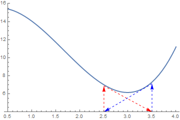
Finally, there is a chance that Newton's method will cycle back and forth between two value and never converge at all. This failure is illustrated in the Figure below.
a1 = {Arrowheads[Medium], Arrow[{{2.5, 6.875}, {3.5, 4}}]}
a2 = {Arrowheads[Medium], Arrow[{{3.5, 7.125}, {2.5, 4}}]} b1 = Graphics[{Dashed, Red, a1}] b2 = Graphics[{Dashed, Blue, a2}] f[x_] = x^3 - 5*x^2 + 3.05*x + 15 graph = Plot[f[x], {x, 0.5, 4}, PlotRange -> {4, 16}, PlotStyle -> Thick] v1 = {Arrowheads[Medium], Arrow[{{2.5, 4}, {2.5, 6.875}}]} v2 = {Arrowheads[Medium], Arrow[{{3.5, 4}, {3.5, 7.125}}]} b11 = Graphics[{Dashed, Red, v1}] b22 = Graphics[{Dashed, Blue, v2}] Show[graph, b1, b2, b11, b22] |
|
| Newton's method may loop. | Mathematica code |
For example, take a function \( f(x) = x^2 -2x +1 \) and start with x0 =0. The first iteration produces 1 and the second iteration returns back to 0, so the sequence will oscillate between the two without converging to a root. Newton's method diverges for the cube root, which is continuous and infinitely differentiable, except for x = 0, where its derivative is undefined.
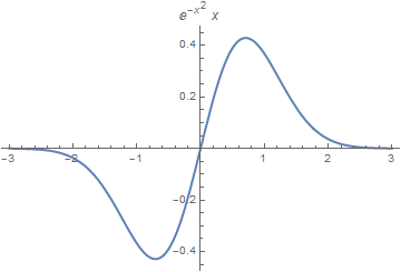
Example 4: This example is a cautionary one. Consider the function \( f(x) = x\,e^{-x^2} \) that obviously has a root at x = 0. However, if your starting point exceeds the root of the equation \( f'(x) = 0 , \) which is \( x_0 = 1/\sqrt{2} \approx 0.707107 , \) then Newton's algorithm diverges.
|
Finally, there is a chance that Newton's method will cycle back and forth between two values and never converge at all. This failure is illustrated in Figure below.
f[x_]= x*Exp[-x^2]
D[x*Exp[-x^2], x] FindRoot[E^-x^2 - 2 E^-x^2 x^2 == 0, {x, 1}] Plot[x*Exp[-x^2], {x, -3, 3}, PlotStyle -> Thick, PlotLabel -> x*Exp[-x^2]] p[0] = 0.8 Do[Print["k= ", k, " " , "p= " , p[k] = p[k - 1] - p[k - 1]/(1 - 2*p[k - 1])], {k, 1, 15}] |
|
| Graph of the exponential function. | Mathematica code |
The derivative of f(x) is zero at \( x = 1/\sqrt{2} \approx 0.707107 , \) and negative for x > 0.707107.
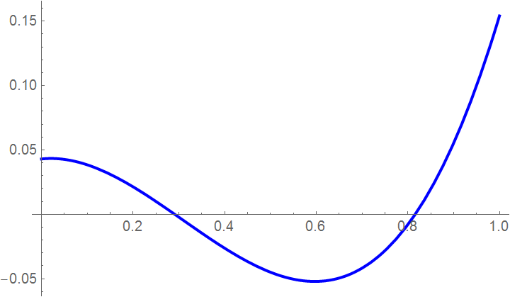
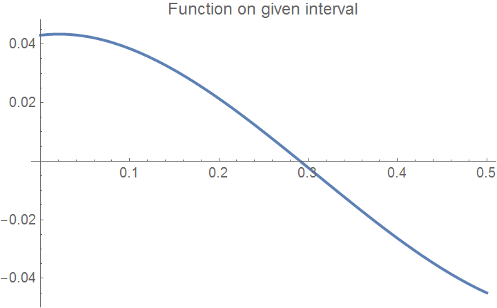
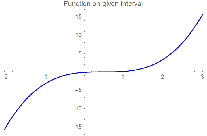
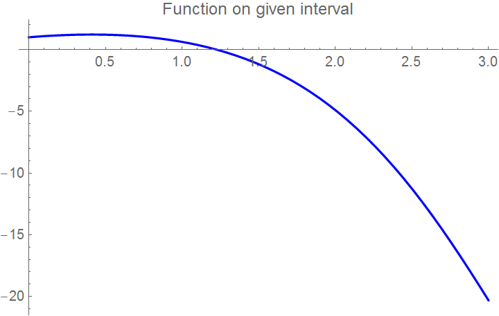
Example 5: Consider the cubic function \( f(x) = x^3 - 0.926\,x^2 + 0.0371\,x + 0.043 . \) First we plot the function, and then define the range of 'x' where you want to see its null.
Plot[f[x], {x, 0, 1}, PlotStyle -> {Thick, Blue}]
xbegin = 0; xend = 0.5;
curve = Plot[f[x], {x, xbegin, xend}, PlotLabel ->
"Function on given interval", PlotStyle -> {Thick, FontSize -> 11}]
 |
 |
step = (xend - xbegin)/10;
Do[ If[f[i] > maxi, maxi = f[i]];
If[f[i] < mini, mini = f[i]], {i, xbegin, xend, step}];
tot = maxi - mini
mini = mini - 0.1*tot; maxi = maxi + 0.1*tot;
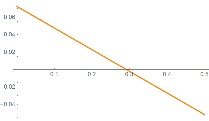
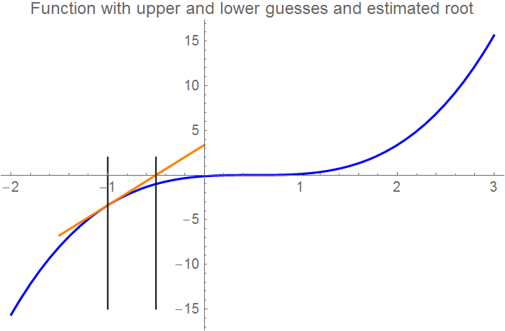
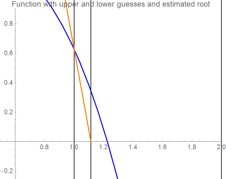
tline = Plot[tanline[x], {x, xbegin, xend}, PlotStyle -> {Thick, Orange}]
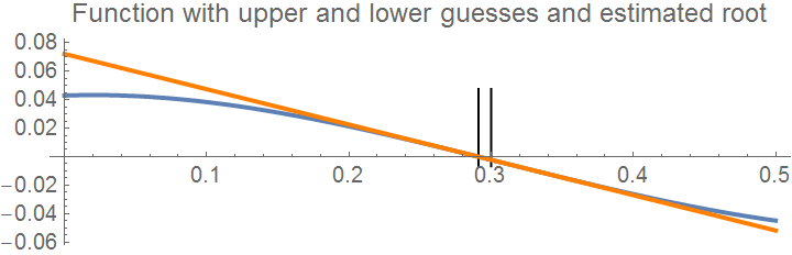
Show[Graphics[Line[{{x0, maxi}, {x0, mini}}]], curve,
Graphics[Line[{{x1, maxi}, {x1, mini}}]], tline, Axes -> True,
PlotLabel -> "Function with upper and lower guesses and estimated root", PlotStyle -> {FontSize -> 10}]
 |
 |
NumberForm[N[s], 20]
Example 6: We reconsider the function \( f(x) = e^x\, \cos x - x\, \sin x \) that has one root within the interval [0,3]. We define the range of x:
step = (xb - xa)/10;
x[0] = xa;
Do[ x[i] = x[i - 1] + step; If[f[x[i]] > maxi, maxi = f[x[i]]; If[f[x[i]] < mini, mini = f[x[i]]]];
Print["i= ", i, ", x[i]= ", x[i], ", f[x[i]]= ", N[f[x[i]]]]; , {i, 1, 10}]
g[x_] := f'[x]
actual = x /. s
NumberForm[N[actual], 20]
Array[xr, nmaximum];
xr[i] = xr[i - 1] - f[xr[i - 1]]/g[xr[i - 1]]]
For[i = 1, i <= nmaximum, i++, Et[i] = Abs[actual - xr[i]]]
For[i = 1, i <= nmaximum, i++, et[i] = Abs[Et[i]/actual*100]]
For[i = 1, i <= nmaximum, i++,
If[i <= 1, Ea[i] = Abs[xr[i] - x0], Ea[i] = Abs[xr[i] - xr[i - 1]]]]
For[i = 1, i <= nmaximum, i++, ea[i] = Abs[Ea[i]/xr[i]*100]]
For[i = 1, i <= nmaximum, i++,
If[(ea[i] >= 5) || (i <= 1), sigdig[i] = 0,
sigdig[i] = Floor[(2 - Log[10, Abs[ea[i]/0.5]])]]]
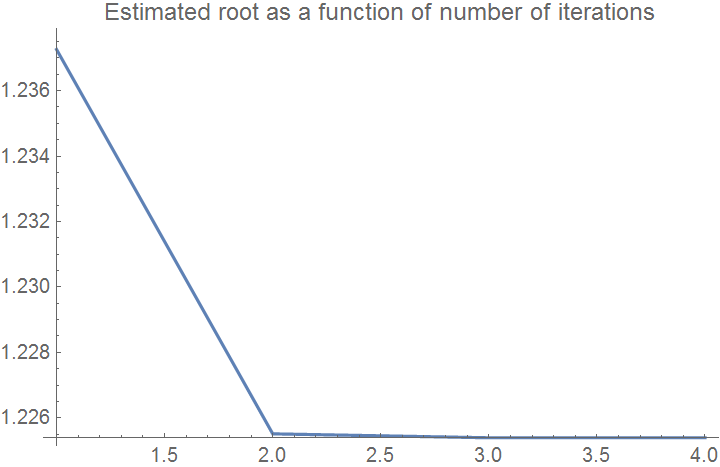
ListPlot[xrplot, Joined -> True, PlotRange -> All,
AxesOrigin -> {1, Min[xrplot]},
PlotLabel -> "Estimated root as a function of number of iterations"]
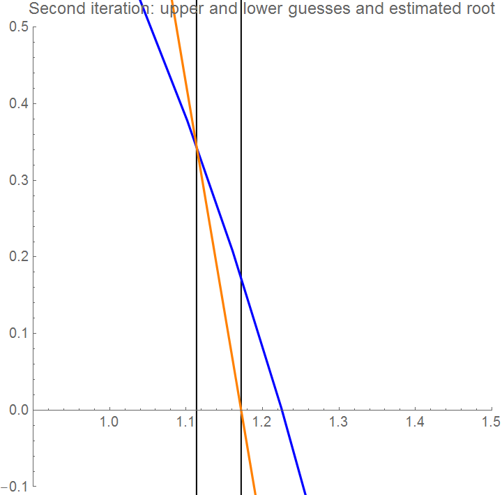
Example 7: This example shows that Newton's method may converge slowly due to an inflection point occurring in the vicinity of the root. Let us consider the function \( f(x) = (x-0.5)^3 . \) First we define the function and its derivative:
g[x_] := f'[x]
curve = Plot[f[x], {x, xbegin, xend},
PlotLabel -> "Function on given interval", PlotStyle -> {FontSize -> 11, Blue}]
tline = Plot[tanline[x], {x, -1.5, 0.0}, PlotStyle -> {Orange}];
Show[curve, tline, Graphics[Line[{{x0, 2}, {x0, -15}}]],
Graphics[Line[{{x1, 2}, {x1, -15}}]], Axes -> True, PlotRange -> All,
PlotLabel -> "Function with upper and lower guesses and estimated root", PlotStyle -> {FontSize -> 10}]
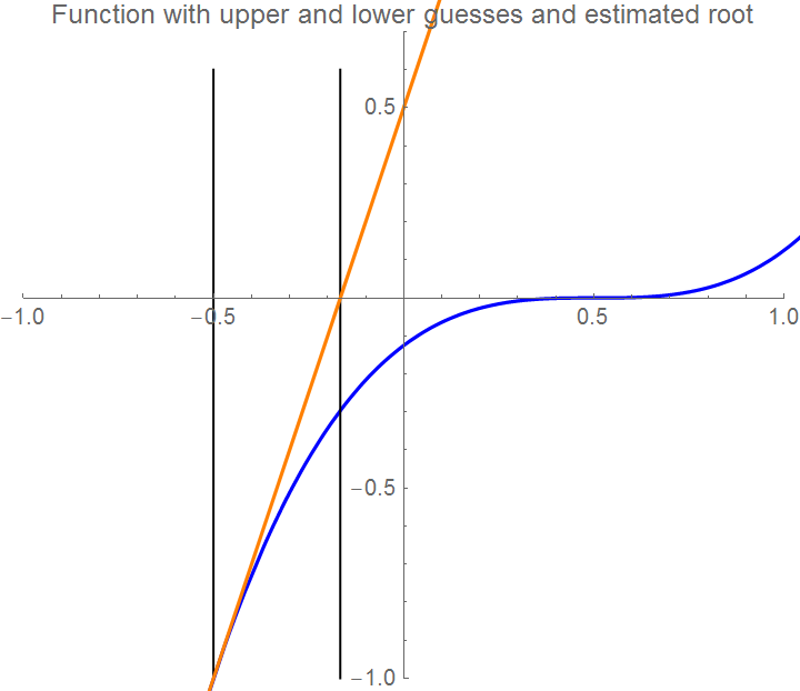
tline = Plot[tanline[x], {x, -1, 1}, PlotStyle -> {Orange}];
Show[Graphics[Line[{{x1, 0.6}, {x1, -1}}]], curve,
Graphics[Line[{{x2, 0.6}, {x2, -1}}]], tline, Axes -> True,
PlotLabel -> "Second iteration and estimated root", PlotStyle -> {FontSize -> 10}, PlotRange -> {{-1, 1}, {-1, 0.7}}]
|
\[
x_{k+1} = x_k - \frac{f(x_k)}{f' (x_k ) - p\,f (x_k )} , \qquad k=0,1,2,\ldots ;
\tag{Newton.3}
\]
|
|---|
where p is a real number. This algorithm coincides with Newton's method for p = 0, and it is of order 2 for general p. However, for \( \displaystyle p = \frac{f'' (x_k )}{2\,f' (x_k )} \) it is of order 3 and it is known as Halley's method.
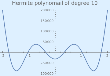
Example: Consider the Hermite polynomial of degree 10:
|
We plot the Hermite polynomial with the following Mathematica code:
Plot[HermiteH[10, x], {x, -2, 2}, PlotStyle -> Thick,
PlotLabel ->
Style["Hermite polynomial of degree 10", FontSize -> 16],
Background -> LightBlue]
|
|
| Hermite polynomial of degree 10. | Mathematica code |
Since these polynomials were discovered by P.Chebyshev, they are called also Chebyshev--Hermite polynomials. Since the Hermite polynomial has negative value at x = 0
II. Secant method
A palpable drawback of Newton's method is that it requires us to have a formula for the derivative of f. For classroom examples this is not an issue, but in the "real world" it can be. Suppose, for example, that f is instead "defined" by a separate subprogram that uses about 1,000 lines of involved computer code. Even if we could theoretically write a formula for the derivative from which f' could be constructed, is this a practical task to set for ourselves?
One obvious way to deal with this problem is to use an approximation to the derivative with the Newton formula
|
\[
x_{k+1} = x_k - \frac{f(x_k ) \left( x_k - x_{k-1} \right)}{f (x_k ) - f(x_{k-1} )} = \frac{x_{k-1} f (x_k ) - x_k f(x_{k-1} )}{f (x_k ) - f(x_{k-1} )}, \qquad k=0,1,2,\ldots .
\tag{Secant.1}
\]
|
|---|
|
plot = Plot[0.7*x^2, {x, 0, 2}, AspectRatio -> 1,
PlotStyle -> {Thickness[0.01], Blue}, Axes -> False,
Epilog -> {PointSize[0.03], Pink, Point[{{0, 0}, {2, 2.8}}]},
PlotRange -> {{-0.5, 2.2}, {-0.2, 4.4}}];
line = Graphics[{Thick, Dashed, Black, Line[{{0, 0}, {2, 2.8}}]}]; arrow = Graphics[{Arrowheads[0.07], Arrow[{{-0.2, 0.3}, {2.2, 0.3}}]}]; l1 = Graphics[{Thick, Dashed, Line[{{0, -0.1}, {0, 0.3}}]}]; l2 = Graphics[{Thick, Dashed, Line[{{0.22, 0.03}, {2, 2.8}}]}]; l3 = Graphics[{Thick, Dashed, Line[{{2, 0.3}, {2, 2.8}}]}]; l4 = Graphics[{Thick, Dashed, Line[{{0.22, 0.03}, {0.22, 0.3}}]}]; l5 = Graphics[{Thick, Dashed, Line[{{0.4, 0.11}, {0.4, 0.3}}]}]; l6 = Graphics[{Thick, Dashed, Line[{{0.4, 0.11}, {2, 2.8}}]}]; t1 = Graphics[{Black, Text[Style[Subscript[x, 0], 16], {0, 0.45}]}]; t2 = Graphics[{Black, Text[Style[Subscript[x, 1], 16], {2, 0.2}]}]; t3 = Graphics[{Black, Text[Style[Subscript[x, 2], 16], {0.22, 0.45}]}]; t4 = Graphics[{Black, Text[Style[\[Alpha], 16], {0.7, 0.23}]}]; t5 = Graphics[{Black, Text[Style[Subscript[x, 3], 16], {0.4, 0.45}]}]; t8 = Graphics[{Black, Text[Style["f(b)", {1.08, 1}]]}]; t8 = Graphics[{Black, Text[Style["f(b)", {1.08, 1}]]}]; Show[arrow, plot, line, l1, l2, l3, l4, l5, l6, t1, t2, t3, t4, t5, t8, t9, Epilog -> {PointSize[0.02], Purple, Point[{{0, 0}, {0, 0.3}, {0.22, 0.3}, {0.22, 0.03}, {0.4, 0.3}, {0.4, 0.11}, {0.52, 0.3}, {2, 0.3}}]}] |
|
| Secant algorithm. | Mathematica code |
The Secant algorithm can be implemented in Mathematica:
NestList[Last[#] - {0, (Function[x, f][Last[#]]*
Subtract @@ #)/Subtract @@ Function[x, f] /@ #}&, {x0, x1}, n]
The secant method is consistent with Newton's method, and its error is proportional to h = xk+1 - xk. Thus, if we assume that the iteration is converging (so that h = xk+1 - xk → 0), then the secant method becomes more and more like Newton's method. Hence, we expect rapid convergence of the secant iterates near the root α. The secant method has a number of advantages over Newton's method. Not only does it not require the derivative, but it can be coded in such a way as to require only a single function evaluation per iteration. Newton requires two: one for the function and one for the derivative. Thus, the secant method is about half as costly per step as Newton's method.
When the secant method is applied to find a square root of a positive number A, we get the formula
|
\[
p_{k+1} = p_k - \frac{p_k^2 -A}{p_k + p_{k-1}} , \qquad k=1,2,\ldots .
\tag{Secant.2}
\]
|
|---|
Print["p0=",PaddedForm[p0,{16,16}]", f[p0]=",NumberForm[f[p0],16]];
Print["p1=", PaddedForm[p1,{16,16}],", f[p1]=", NumberForm[f[p1],16]];
p2=p1; p1=p0;
While[k < max, p0=p1;p1=p2; p2=p1-(f[p1](p1-p0))/(f[p1]-f[p0]);
k=k+1;
Print["p "k, "=", PaddedForm[p2,{16,16}],", f[","p"k,"]=",NumberForm[f[p2],16]];];
Print["p =",NumberForm[p2,16]];
Print[" Δp=±"Abs[p2-p1]];
Print["f[p]=",NumberForm[f[p2],16]];]
Input: x0 and x1
Set y0=f(x0) and y1=f(x1)
Do
   x=x1-y1*(x1-x0)/(y1-y0)
   y=f(x)
   Set x0=x1 and x1=x
   Set y0=y1 and y1=y
Until |y1| < tol
Example 8: Let us find a positive square root of 6. To start secant method, we need to pick up two first approximations,which we choose by obvious bracketing: \( x_0 =2, \quad x_1 =3 . \)
Example 9: We consider the function \( f(x) = e^x\, \cos x - x\, \sin x \) that has one root within the interval [0,3]. We define the range of x:
xa = 0; xb = 3;
PlotLabel -> "Function on given interval", PlotStyle -> {FontSize -> 11, Blue}]
Graphics[Line[{{xguess1, maxi}, {xguess1, mini}}]], Axes -> True,
PlotLabel -> "Function with upper and lower guesses",
PlotStyle -> {FontSize -> 10}, PlotRange -> {{0.7, 2}, {-0.2, 0.4}}]
secantline[x_] = m*x + f[xguess2] - m*xguess2;
sline = Plot[secantline[x], {x, xa, x1}, PlotStyle -> {Orange}]
Show[Graphics[Line[{{xguess2, maxi}, {xguess2, mini}}]],
Graphics[Line[{{x1, maxi}, {x1, mini}}]], curve,
Graphics[Line[{{xguess1, maxi}, {xguess1, mini}}]], sline,
Axes -> True, PlotLabel -> "Function with upper and lower guesses and estimated root",
PlotStyle -> {FontSize -> 10}, PlotRange -> {{0.5, 2}, {-0.25, 0.9}}]
We make the second iteration.
secantline[x_] = m*x + f[x1] - m*x1;
sline = Plot[secantline[x], {x, 1, 1.3}, PlotStyle -> {Orange}]
Show[Graphics[Line[{{xguess2, maxi}, {xguess2, mini}}]],
Graphics[Line[{{x1, maxi}, {x1, mini}}]], curve,
Graphics[Line[{{xguess1, maxi}, {xguess1, mini}}]], sline,
Axes -> True, PlotLabel -> "Function with upper and lower guesses and estimated root",
PlotStyle -> {FontSize -> 10}, PlotRange -> {{0.5, 2}, {-0.25, 0.9}}]
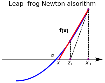
It is possible to combine the secant method and weighed Newton's method:
|
plot = Plot[1*x^2, {x, 0, 1}, AspectRatio -> 1,
PlotStyle -> {Thickness[0.01], Blue}, Axes -> False, Epilog -> {PointSize[0.03], Pink, Point[{{0, 0}, {2, 2.8}}]}, PlotRange -> {{-0.5, 1.2}, {-0.2, 1.4}}]; arrow = Graphics[{Arrowheads[0.07], Arrow[{{-0.2, 0.3}, {1.2, 0.3}}]}]; l1 = Graphics[{Thick, Dashed, Line[{{1, 1}, {0.75, 0.3}}]}]; l2 = Graphics[{Thickness[0.01], Red, Line[{{1, 1}, {0.59, 0.3}}]}]; l3 = Graphics[{Thick, Dashed, Line[{{1, 1}, {1, 0.3}}]}]; l4 = Graphics[{Thick, Dashed, Line[{{0.75, 0.55}, {0.75, 0.3}}]}]; t2 = Graphics[{Black, Text[Style[Subscript[x, 0], 16], {1, 0.25}]}]; t3 = Graphics[{Black, Text[Style[Subscript[z, 1], 16], {0.75, 0.25}]}]; t4 = Graphics[{Black, Text[Style[Subscript[x, 1], 16], {0.6, 0.25}]}]; t5 = Graphics[{Black, Text[Style[\[Alpha], 16], {0.5, 0.35}]}]; t9 = Graphics[{Black, Text[Style["f(x)", Bold, 16], {0.66, 0.7}]}]; Show[arrow, plot, l1, l2, l3, l4, t2, t3, t4, t5, t9, Epilog -> {PointSize[0.02], Purple, Point[{{0.6, 0.3}, {0.75, 0.555}, {0.75, 0.3}, {1, 0.3}, {1, 1}}]}, PlotLabel -> "Leap-frog Newton alsorithm", LabelStyle->{FontSize->16,Black} ] |
|
| Leap-frog Newton's algorithm. | Mathematica code |
The following code was prepared by the Computational Class Notes for this website:
{f, x, z, p} = args;
z = x - (f[x]/(f'[x] - p*f[x]));
x2 = x - f[x]*((z - x)/(f[z] - f[x]));
{f, x2, z, p} ];
f function,
x0 starting value,
p parameter,
threshold for when to stop,
s is scale of the horizontal axes to scale around converging limit,
syms are the names of the variables for f
Module[{z, list, polyline, len, polylinezoom, dataset},
list = {};
z = (x - (f[x]/(f'[x] - p*f[x]))) /. {x -> x0};
FixedPointList[(AppendTo[list, {#, leapfrog[#]}]; leapfrog[#]) &, {f, x0, z, p}, SameTest -> (Norm[#1 - #2] < threshold &)];
polyline = Flatten[Table[{
{list[[i]][[1]][[2]], 0.0},
{list[[i]][[1]][[2]], f[list[[i]][[1]][[2]]]},
{list[[i]][[2]][[3]], 0},
{list[[i]][[2]][[3]], f[list[[i]][[2]][[3]]]}
}, {i, 1, Length@list}], 1];
len = Ceiling[(Length@polyline)/3];
If[len > 8, polylinezoom = Take[polyline, -len], polylinezoom = polyline];
dataset = Dataset[Table[
<|
syms[[1]] -> (polyline[[i]][[1]]),
syms[[2]] -> (polyline[[i]][[2]]) , If[
i > 1 && i < Length@polyline, ("\[CapitalDelta]" <> syms[[1]]) ->
Abs[polyline[[i]][[1]] - polyline[[i + 1]][[1]]], ("\[CapitalDelta]" <> syms[[1]]) -> ("")],
If[i > 1 && i < Length@polyline, ("\[CapitalDelta]" <> syms[[2]]) ->
Abs[polyline[[i]][[2]] - polyline[[i + 1]][[2]]],
("\[CapitalDelta]" <> syms[[2]]) -> ("")]
|>, {i, 1, Length@polyline}]];
<|
"list" -> list, "f" -> TraditionalForm[f["x"]], "x0" -> x0, "p" -> p, "poly line" -> polyline, "table" -> dataset, "plot" -> Show[ { Graphics[{Dotted, Line@polyline }, Ticks -> {{#, Rotate[#, Pi/2]} & /@ polyline[[All, 1]], None}, AxesStyle -> Directive[Gray, FontSize -> 8], AxesLabel -> {syms[[1]], Row@{syms[[2]], "=", TraditionalForm[f[syms[[1]]]]}}], Plot[f[x], {x, Min[polyline[[All, 1]]] - 0.1, Max[polyline[[All, 1]]] + 0.1}, Axes -> True, AxesLabel -> {syms[[1]], Row@{syms[[2]], "=", TraditionalForm[f[syms[[1]]]]}}, PlotStyle -> Opacity[0.3]] }, Axes -> True, PlotRange -> {{Min[polyline[[All, 1]]] - 0.1, Max[polyline[[All, 1]]] + 0.1}, {Min[polyline[[All, 2]]] - 0.2, Max[polyline[[All, 2]]] + 0.2}} ], "plot zoom" -> Show[ { polylinezoom = (#*{1, s}) & /@ polylinezoom; Graphics[{Dotted, Line@polylinezoom }, Ticks -> {{#, Rotate[#, Pi/2]} & /@ polylinezoom[[All, 1]], None}, AxesStyle -> Directive[Gray, FontSize -> 8], AxesLabel -> {syms[[1]], Row@{syms[[2]], "=", TraditionalForm[f[syms[[1]]]]}}], Plot[s*f[x], {x, Min[polylinezoom[[All, 1]]] - 0.0, Max[polylinezoom[[All, 1]]] + 0.0}, Axes -> True, AxesLabel -> {syms[[1]], Row@{syms[[2]], "=", TraditionalForm[f[syms[[1]]]]}}, PlotStyle -> Opacity[0.3]] }, Axes -> True, AxesOrigin -> {Min[polylinezoom[[All, 1]]], 0}, PlotRange -> {{Min[polylinezoom[[All, 1]]] - 0.0, Max[polylinezoom[[All, 1]]] + 0.0}, {Min[polylinezoom[[All, 2]]] - 0.0, Max[polylinezoom[[All, 2]]] + 0.0}} ] |> ]; f[w_] := (w - 100)^2; p = 0.1; x0 = 102.0; threshold = 1*^-3; res = leapfrogFIXEDPOINT[f, x0, p, threshold, 500, {"t", "x"}];
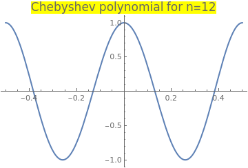
Example 10: Consider the Chebyshev polynomial of the first kind that is the solution of the initial value problem
|
Plot[ChebyshevT[12, x], {x, -0.5, 0.5}, PlotStyle -> Thick,
Then we write the code based on leap-frog Newton algorithm
PlotLabel -> Style["Chebyshev polynomial for n=12", FontSize -> 16, Background -> Yellow]]
f[x_] = ChebyshevT[12, x]; f1[x_] = D[f[x], x];
RecurrenceTable[{x[k + 1] == x[k] - (z[k] - x[k])*f[x[k]]/(f[z[k]] - f[x[k]]), z[k + 1] == x[k] - f[x[k]]/f1[x[k]], x[0] == 0.1, z[0] == 0.1 - f[0.1]/f1[0.1]}, {x, z}, {k, 0, 5}]// Grid
{{0.1, 0.132044}, {0.13049, 0.132044}, {0.130526,
0.130526}, {0.130526, 0.130526}, {0.130526, 0.130526}, {0.130526,
0.130526}}
ListPlot[%, PlotRange -> All]
|
|
| Chebyshev polynomial of the first kind. | Mathematica code |
So we see that three iterations are need to obtain six digit accuracy root: 0.130526. ■
III. Steffensen's Iteration Method
Suppose that we need to find a root α of a smooth function f, so f(α) = 0. Given an adequate starting value x0, a sequence of values x1, x2, … , xn, … can be generated using the Steffensen's formula below
|
\[
x_{k+1} = x_k - \frac{f^2 \left( x_k \right)}{f \left( x_k + f \left( x_k \right) \right) - f \left( x_k \right)} , \qquad k=0,1,2,\ldots .
\tag{Steffensen.1}
\]
|
|---|
Johan's revolutionary idea is based on applying Newton's iteration scheme but replacing the derivative in (Newton.1) by the forward approximation: \( \displaystyle f' \left( x_k \right) \approx \frac{f \left( x_k + f( x_k )\right) - f \left( x_k \right)}{ f \left( x_k \right)} = \frac{f\left( x_k + h \right) - f\left( x_k \right)}{h} ,\) where h = f(xk) plays the role of the infinitesimal increment, which is close to zero when xk is near the root α. Now it is clear why Steffensen's method is very sentitive to the initial quess value x0 because f(x0) must be very small. However, a more accurate approximation is obtained by utilizing a symmetric difference quotient
Note that only the head of the function is specified when it is passed to the SteffensonMethod subroutine. Steffensen's algorithm can be implemented within the Wolfram language with the aid of NestWhileList command. The nesting iteration will be terminated when the last two iterates become the same, but no more than 20 times (by default n ≤ 20):
Although Steffensen's method works very well, because of machine limitations, there could be situations when the denominator may lose significant places due to subtraction of two almost equal floating point terms. To avoid such situations, Steffensen's algorithm can be modified with either Aitken's delta-squared process or introducing a real parameter p:
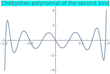
Example 11: Consider the Chebyshev polynomial of the second kind that is the polynomial solution of the initial value problem
|
Plot[ChebyshevU[11, x], {x, -1, 1}, PlotStyle -> Thick,
PlotLabel -> Style["Chebyshev polynomial of the second kind", FontSize -> 16, Background -> Cyan]] |
|
| Chebyshev polynomial of the second kind. | Mathematica code |
First, we bracket a positive root of the Chebyshev polynomial:
We make a few steps manually to see how Steffensen's algorithm works. With an initial approximation x0 = 0.3, we get
x1 = a - p0^2/(ChebyshevU[11, a + p0] - p0)
i = 1; NN = 30; tol = 1/10^7; p0 = N[f[a]]; p02 = p0*p0; x0 = a;
While[i < NN,
x1 = x0 - 2*p02/(f[x0 + p0] - f[x0 - p0]);
x0 = x1; p0 = N[f[x0]]; p02 = (f[x0])^2;
Print["i= ", i, ", x= ", x1, ", f= ", p0]; i++]
On the first step, we get
x2 = x1 - p02/(ChebyshevU[11, x1 + p0] - p0 - 6*p02)
x3 = x2 - p02/(ChebyshevU[11, x2 + p0] - p0 - 6*p02)
We write a loop:
i = 1; NN = 5; tol = 1/10^7; p0 = N[f[a]]; p02=p0*p0; x0 = a;
While[i < NN,
x1 = x0 - p02/(f[x0 + p0] - p0 - 6*p02);
x0 = x1; p0 = N[f[x0]]; p02 = (f[x0])^2;
Print["i= ", i, ", x= ", x1, ", f= ", p0]; i++
]
i = 1; NN = 5; tol = 1/10^7; p0 = N[f[a]]; p02=p0*p0; x0 = a;
While[i <= NN,
z1 = x0 - p02/(f[x0 + p0] - p0 - 6*p02);
x1=x0 - (z1-x0)*p0/(f[z1]-p0);
x0 = x1; p0 = N[f[x0]]; p02 = (f[x0])^2;
Print["i= ", i, ", x= ", x1, ", f= ", p0]; i++
]
We compare our results with Newton's method (Newton.1):
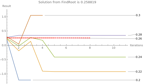
Now we investigate the sensitivity of Steffensen's algorithm to the starting value. Utilizing ListLinePlot facilitates to see how quickly the solution stabilizes. The dashed thick red line shows the solution as determined by Mathematica built-in command FindRoot.
|
(* making a list of some starting values *)
x0List = Range[0.2, 0.3, 0.02]
{0.2, 0.22, 0.24, 0.26, 0.28, 0.3}
Then we map the function across the list of starting values.
The maximum number of iterations is 10 simply for aesthetic purposes.
root = FindRoot[f[x], {x, 0.3}];
ListLinePlot[ SteffensonMethod2[f, #, 10] & /@ x0List, (* the root determined by FindRoot is shown as a thick red dashed line *) Epilog -> {Thick, Dashed, Red, Line[{{1, x}, {8, x}}] /. root}, (* Adding labels, legends, making the plot look nicer *) PlotLabels -> x0List, ImageSize -> Large, AxesLabel -> {"Iterations", "Result"}, PlotRange -> {{1, Automatic}, Automatic}, PlotLegends -> x0List, PlotLabel -> "Solution from FindRoot is " <> ToString[x /. root] ] |
|
| Sensitivity of Steffensen's algorithm to the starting value. | Mathematica code |
■
IV. Chebyshev Iteration Scheme
|
\[
x_{k+1} = x_k - \frac{f \left( x_k \right)}{f' \left( x_k \right)} - \frac{f^2 \left( x_k \right) f'' \left( x_k \right)}{2\left( f' \left( x_k \right)
\right)^3} , \qquad k=0,1,2,\ldots .
\tag{Chebyshev.1}
\]
|
|---|
NestList[# - Function[x, f][#]/Derivative[1][Function[x, f]][#] -
Function[x, f^2][#]* Derivative[2][Function[x, f]][#]/
2/(Derivative[1][Function[x, f]][#])^3 &, x0, n]
|
\[
p_{k+1} = \frac{1}{2} \left( p_k + \frac{A}{p_k} \right) - \frac{\left( p_k^2 -A \right)^2}{8\,p_k^3} , \qquad k=0,1,2,\ldots .
\tag{Chebyshev.2}
\]
|
|---|
Example 12: Let us reconsider the problem of determination of a positive square root of 6 using Chebyshev iteration scheme:
Do[Print["k= ", k, " " , "p= " , p[k] = (p[k - 1] + 6/p[k - 1])/ 2 - (p[k - 1]^2 - 6)^2/(8*p[k - 1]^3)], {k, 1, 5}]
|
\[
x_{k+1} = \frac{2\,x_k^3 +A}{3\,x^2_k} - \frac{x_k \left( x_k^3 - A \right)^2}{9\,x_k^{6}} , \qquad k=0,1,2,\ldots .
\tag{Chebyshev.3}
\]
|
|---|
Example 13: Let us find a root of the Laguerre polynomial L21(x) of order 21 that can be defined by the Rodrigues formula
|
We plot the Laguerre polynomial to identify the interval containing the root.
Plot[LaguerreL[21, x], {x, 0, 3}, PlotStyle -> {Thick, Magenta}]
|
|
| Graph of the Laguerre polynomial L21(x). | Mathematica code |
Since these polynomials were discovered by P.Chebyshev, they are called also Chebyshev--Laguaere polynomials, after Edmond Laguerre (1834–1886).
To find its first positive root, we use the standard Mathematica command
V. Halley's Method
|
\[
x_{k+1} = x_k - \frac{f\left( x_k \right)}{f'\left( x_k \right)} - \frac{f \left( x_k \right) f'' \left( x_k \right)}{2\left( f' \left( x_k \right)\right)^2 - f \left( x_k \right) f'' \left( x_k \right) } \cdot \frac{f\left( x_k \right)}{f'\left( x_k \right)} = x_k - \frac{2\,f \left( x_k \right) f' \left( x_k \right)}{2\left( f' \left( x_k \right)\right)^2 - f \left( x_k \right) f'' \left( x_k \right) }
, \qquad k=0,1,2,\ldots . \tag{Halley.1}
\]
|
|---|
NestList[# - Function[x, f][#]/Derivative[1][Function[x, f]][#] -
Function[x, f^2][#]* Derivative[2][
Function[x, f]][#]/(2*(Derivative[1][Function[x, f]][#])^2 -
Function[x, f][#] * Derivative[2][Function[x, f]][#])/
Derivative[1][Function[x, f]][#] &, x0, n]
|
\[
x_{k+1} = \frac{1}{2} \left( x_k + \frac{A}{x_k} \right) - \frac{\left( x_k^2 -A \right)^2}{2x_k \left( 3\,x_k^2 + A \right)} , \qquad k=0,1,2,\ldots .
\tag{Halley.2}
\]
|
|---|
There is another version of the preceding algorithm that is of order 3 and it is called the super-Halley:
|
\[
x_{k+1} = x_k - \frac{f\left( x_k \right)}{f'\left( x_k \right)} -
\frac{f(x_k )\, f'' (x_k )}{\left( f' (x_k ) \right)^2 - f(x_k )\, f'' (x_k )} \cdot \frac{f\left( x_k \right)}{2\,f'\left( x_k \right)} , \qquad k=0,1,2,\ldots . \tag{Halley.3}
\]
|
|---|
NestList[# - Function[x, f][#]/Derivative[1][Function[x, f]][#] -
Function[x, f^2][#]* Derivative[2][Function[x, f]][#]/
2/((Derivative[1][Function[x, f]][#])^2 -
Function[x, f][#] * Derivative[2][Function[x, f]][#])/
Derivative[1][Function[x, f]][#] &, x0, n]
|
\[
x_{k+1} = \frac{1}{2} \left( x_k + \frac{A}{x_k} \right) - \frac{\left( x_k^2 -A \right)^2}{4x_k \left( x_k^2 + A \right)} , \qquad k=0,1,2,\ldots .
\tag{Halley.4}
\]
|
|---|
Example 14: Let us find a few iterations for determination of a square root of 6:
Do[Print["k= ", k, " " , "p= " , p[k] = p[k - 1] - 2*p[k - 1]*(p[k - 1]^2 - 6)/(3*p[k - 1]^2 + 6)], {k, 1, 5}]
Example 15: Let us find a root of the Legendre polynomial P20(x) of order 20 that can be defined by the Rodrigues formula
|
Legendre polynomials are named after Adrien-Marie Legendre (1752--1833), who discovered them in 1782.
We plot the Legendre polynomial to identify the interval containing the root.
Plot[LegendreP[20, x], {x, 0, 3}, PlotStyle -> {Thick, Magenta}]
|
|
| Graph of the Legendre polynomial P20(x). | Mathematica code |
First, we find the third positive zero of the Legendre polynomial with the aid of Mathematica standard command
VI. Dekker's Method

As we saw previously, combination of different iteration algorithms may lead to acceleration of convergence or make it more robust. It was a Dutch mathematician, called Theodorus Jozef Dekker (born in 1927), who proposed an algorithm in 1960 to combine the open iterative method (not restricted to an interval, but usually converges quickly without any guarantee of finding a root) and the closed iterative method (that uses a bounded interval and usually converges slowly to a root if it exists). In particular, he suggested to alternate the robust bisection method (which is slow in computations) with the fast open end secant iterative algorithm. Unfortunately, his original paper is not available on the web, but his next paper published with J.Bus in 1975 can be seen on the Internet. Theodorus Jozef Dekker completed his Ph.D degree from the University of Amsterdam in 1958. Later, Dekker's method was modified, and its latest version, known as Brent or van Wijngaarden--Dekker--Brent method is discussed in the next subsection. Our presentation provides a rough outline of the basic algorithm and does not include possible improvements.
The advantages of Dekker's method were outlined by the founder of the computer science department at Stanford university George E. Forzythe (who was a Ph.D adviser of Cleve Moler, an inventor of matlab):
- it is as good as the bisection method, so it always converges to the root;
- there are no assumptions about the second derivative of the function;
- it is as fast as the secant method;
- it is not concerned with multiple roots unlike the secant method.
Suppose that we want to solve the equation f(x) = 0, where f: ℝ → ℝ is a smooth real-valued function. As with the bisection method, we need to initialize Dekker's method with two points, say 𝑎0 and b0, such that \( f \left( a_0 \right) \quad\mbox{and} \quad f \left( b_0 \right) \) have opposite signs. If f is continuous on \( \left[ a_0 , b_0 \right] , \) the intermediate value theorem guarantees the existence of a solution between a0 and b0.
The Algorithm
Two points are involved in every iteration: 𝑎 and b, where b is the current guess for the root α of f(x).
- Dekker's method starts with two points that embrace a root α, for which f(α) = 0. So there exists an interval that includes the root: α ∈ [𝑎, b], with f(𝑎) × f(b) < 0.
- 𝑎k is the "contrapoint," i.e., a point such that \( f \left( a_k \right) \quad\mbox{and} \quad f \left( b_k \right) \) have opposite signs, so the interval \( \left[ a_k , b_k \right] \) contains the solution. Furthermore, \( \left\vert f \left( b_k \right) \right\vert \) should be less than or equal to \( \left\vert f \left( a_k \right) \right\vert , \) so that bk is a better guess for the unknown solution than 𝑎k.
-
At every step of iteration, the following conditions are maintained:
\[ f\left( a_k \right) \times f\left( b_k \right) \le 0, \quad \left\vert f\left( b_k \right) \right\vert \le \left\vert f\left( a_k \right) \right\vert , \quad \left\vert a_k - b_k \right\vert \le 2\,\delta (b) , \]where δ is the required tolerance.
- bk-1 is the previous iterate (for the first iteration, we set bk-1 = 𝑎0).
-
Calculate two values: one using the secant method
\[ s = b_k - \frac{b_k - b_{k-1}}{f\left( b_k \right) - f\left( b_{k-1} \right)}\, f\left( b_k \right) , \qquad \mbox{if } f\left( b_k \right) \ne f\left( b_{k-1} \right) , \]and another midpoint\[ m = \frac{f(a_k ) + f(b_k )}{2} \qquad \mbox{if } f\left( b_k \right) = f\left( b_{k-1} \right) . \]
- If the value s from the secant algorithm lies strictly between bk and m, then it becomes the next iterate: bk+1 = s.
- Otherwise, bk+1 = m.
- The new contrapoint is chosen such that f(𝑎k+1) and f(bk+1) have opposite signs. If f(𝑎k) and f(bk+1) have opposite signs, then the contrapoint remains the same: 𝑎k+1 = 𝑎k. Otherwise, f(bk+1) and f(bk) have opposite signs, so the new contrapoint becomes 𝑎k+1 = bk.
- Finally, if |f(𝑎k+1)| < |f(bk+1)|, then 𝑎k+1 is probably a better guess for the required zero than bk+1, and hence the values of 𝑎k+1 and bk+1 are swapped.
Example 16: We demonstrate the Dekker's method with the following pathological example for a function that has a singularity. So we consider a problem for finding the inverse value of an arbitrary number 𝑎:
To simplify our job, we set k = 0 and 𝑎 = 1. We embrace the root α = 1 by the interval [0.1, 2]. The function \( f(x) = x^{-1} -1 \) has the following values at its endpoints:
The Dekker method improves the secant method to make it more stable by combining it with the bisection method. This combination allows the Dekker method to converge for any continuous function. For each iteration of the algorithm, the two methods are evaluated. If the estimate of the root obtained by the secant method lies between the last value calculated by the algorithm and the new estimate obtained by the bisection method, the value of the secant method is used as one of the boundaries for the next iteration. If not, it may indicate that the secant method is diverging and the bisection iteration value is used as a boundary for the next iteration. The bisection method will need a sign check for the two initial values such that the function values both have the opposite sign, and the Dekker algorithm needs to include this check as well to make sure that the bisection will be a valid method in the next iteration.
Initially, we choose b = 2 and 𝑎 = 0.1 because the value of the function f is smaller at right endpoint. To make the first step, we calculate their mean
s = (a*f[b] - b*f[a])/(f[b] - f[a])
Example 17: Use the Bus--Dekker method to find a root of the equation
|
Plot[Exp[0.1*x]-Exp[0.7*x-1], {x,1,2}, PlotStyle->{Thick, Magenta}]
|
|
| Figure 1: Jordan region for m > 0. | Mathematica code |
We observe that f(1) is positive while f(2) is negative, and hence that there is at least one root in [1,2]. The basis of the Bus--Dekker algorithm is to use the secant method but at the same time ensure a reduction of an interval containing a zero. We start with guesses x = 0 and x = 1.5. Since f(1.5) is positive, we can immediately reduce the interval containing a zero from the initial interval [1,2] to [1.5,2]. So we set b1 = 1.5 and 𝑎 = 2.
b=1.5; a=2;
m = (a+b)/2
m = (a+b)/2
m = (a+b)/2
VII. Brent's Method

Dekker's method performs well if the function f is reasonably well-behaved. However, there are circumstances in which every iteration employs the secant method, but the iterates bk converge very slowly (in particular, \( \left\vert b_k - b_{k-1} \right\vert \) may be arbitrarily small). Dekker's method requires far more iterations than the bisection method in this case. Although this algorithm guarantees the convergence and the asymptotic behavior is completely satisfactory, the number of function evaluations required by this algorithm may be prohibitively large, in particular, when the zero appears to be multiple one.
In 1971, the Australian mathematician Richard Pierce Brent (born in 1946, Melbourne) proposed a modification of Dekker's method. With the additional inclusion of the inverse quadratic interpolation, Brent's root-finding algorithm makes it completely robust and usually very efficient.
The method is the basis of matlab’s fzero routine (see its explanation on Cleve’s Corner). The algorithm tries to use the potentially fast-converging secant method or inverse quadratic interpolation if possible, but it falls back to the more robust bisection method if necessary.
The method underwent several modifications, improvements, and implementations.
Consequently, the algorithm is also known as the van Wijngaarden-Deker-Brent method.
For Brent's original algorithm, the upper bound of the number of function evaluations needed equals (t + 1)² - 2, where t is the number of function evaluations needed by bisection. Later, J.C.P. Bus & T.J. Dekker proposed another modification of Brent's algorithm, but requiring at most 4t function evaluations. This is achieved by inserting steps in which rational interpolation or bisection is performed. Some other variations of Brent's method are known with a similar asymptotic behavior. Our presentation outlines the basic ideas and does not follow any version of Brent's algorithm. The example presented illustrates the Brent's method by showing all steps.
The inverse quadratic interpolation method approximates the function y = f(x) by a quadratic curve that goes through three consecutive points { xi, f(xi) }, i = (k, k-1, k-2). As the function may be better approximated by a quadratic curve rather than a straight line, the iteration is likely to converge more quickly. Such a quadratic approximation follows:
The Algorithm
Three points are involved in every iteration: 𝑎, b, and c, where b is the current guess for the root α of f(x). Since there are many checks at every iteration step, we give only basical ideas involved in Brent's algorithm.
- Brent's method starts with two points that embrace a root α, for which f(α) = 0. So there exists an interval that includes the root: α ∈ [b, c], with f((b) × f(c) < 0.
- Initiation: out of two endpoints that embrace the root α, set b to be that which gives the the smallest function value: |f(b)| ≤ |f(c)|.
-
Set 𝑎 = c and determine a new iterate b by linear (secant) interpolation
\[ b= b_1 = \frac{a\,f(b) - b\,f(a)}{f(b) - f(a)} . \]Then set c to be the previous value of b if the function f changes the sign. If not, swap with 𝑎.
- If the three current points 𝑎, b, and c are distinct, find another point i by inverse quadratic interpolation.
- If it fails, try to compute a secant intercept s using b and c. Test whether s is between b and (3𝑎+b)/4. Otherwise set s = m, the midpoint.
- Since b is the most recent approximation to the root and 𝑎 is the previous value of b, apply the linear interpolation if |f(b)| ≥ |f(𝑎)|. Otherwise, do bisection.
- Make a new estimate of the root using the obtained points through either the bisection, secant, or IQI methods, and set b to that closest to the root. Use bisection when when the condition |s - b| < 0.5 |b - c| fails. Check for convergence at the new calculated value. If reached, end the algorithm.
- Check whether f(new value) and f(b) have different signs. If so, they will be the two estimates for the next iteration. If not, the values would be 𝑎 and the newly calculated value. Refresh values of points so that abs(f(b)) < abs(f(𝑎)).
- Start next iteration.
Brent's method contains many comparisons and conditions that make it complicated to follow. It has various implementations; for instance, Bus & Dekker suggest to insert the bisection method at every 5-th iterate. A great deal of attention has been paid to considerations of floating-point arithmetic (overflow and underflow, accuracy of computed expressions, etc.). Let us outline the main check-in points.
Two inequalities must be simultaneously satisfied: Given a specific numerical tolerance δ if the previous step used the bisection method, the inequality
If the previous step performed interpolation, then the inequality
Also, if the previous step used the bisection method, the inequality
Brent proved that his method requires at most N² iterations, where N denotes the number of iterations for the bisection method. If the function f is well-behaved, then Brent's method will usually proceed by either inverse quadratic or linear interpolation, in which case it will converge superlinearly.
Furthermore, Brent's method uses inverse quadratic interpolation (IQI for short) instead of linear interpolation (as used by the secant method). If \( f(b_k ), \ f(a_k ) , \mbox{ and } f(b_{k-1}) \) are distinct, it slightly increases the efficiency. As a consequence, the condition for accepting i (the value proposed by either linear interpolation or inverse quadratic interpolation) has to be changed: s has to lie between \( \left( 3 a_k + b_k \right) /4 \) and bk.
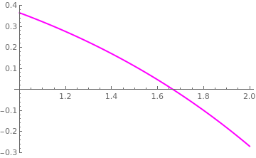
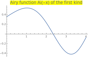
Example 18: Consider the Airy function f(-x) = Ai(-x) of the first kind for negative argument:
|
Plot[AiryAi[-x], {x, 0, 4}, PlotStyle -> Thick,
PlotLabel -> Style["Airy function Ai(-x) of the first kind", FontSize -> 16, Background -> Yellow]] |
|
| Airy function Ai(-x) of the first kind. | Mathematica code |
First, we find the root using the standard Mathematica command
N[f[1]]
A = f[b]*f[c]*a/(a - b)/(a - c) + f[a]*f[c]*b/(b - a)/(b2 - c) + f[a]*f[b]*c/(c - a)/(c - b2)
A = f[b]*f[c]*a/(a - b)/(a - c) + f[a]*f[c]*b/(b - a)/(b2 - c) + f[a]*f[b]*c/(c - a)/(c - b2)
s = (c*f[b] - b*f[c])/(f[b] - f[c])
A = f[b]*f[c]*a/(a - b)/(a - c) + f[a]*f[c]*b/(b - a)/(b - c) + f[a]*f[b]*c/(c - a)/(c - b)
VIII. Ostrowski's Method
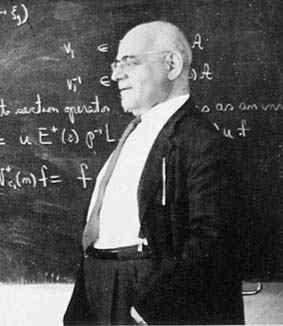
Alexander Markowich Ostrowski (1893---1986) was a talented Russian mathematician who was gifted with a phenomenal memory. Alexander was born to Jewish family in Kiev, Russian Empire. Alexander Ostrowski attended the Kiev College of Commerce, not a high school, and thus had an insufficient qualification to be admitted to university. However, his talent did not remain undetected: Ostrowski's mentor, professor at the University of Kiev, Dmitry Grave, wrote to German mathematicians Edmund Landau (1877--1938) and Kurt Hensel (1861--1941) for help. Subsequently, Ostrowski began to study mathematics at Marburg University in Germany under Hensel's supervision in 1912. When World War I broke out, he was therefore interned as a hostile foreigner. During this period, he was able to obtain limited access to the university library. After the war he resumed his studies at the more prestigious University of Göttingen and was awarded a doctorate in mathematics in 1920. He graduated summa cum laude and worked in different universities. He eventually moved to Switzerland to teach at the University of Basel, before the outbreak of World War II. Ostrowski fared well living in that neutral country during the war. He taught in Basel until he retired in 1958. He remained very active in math until late in his life.
This gifted and prolific mathematician was engaged in various mathematical problems. The advent of computers catapulted Ostrowski to delve into numerical analysis. He studied iterative solutions of large linear systems. Ostrowski passed away in 1986 in Montagnola, Lugano, Switzerland. He had lived there with his wife during his retirement.
Ostrowski tackled the problem of calculating a root for a single-variable non-linear function in a new way. Most of the methods we know perform a single refinement, for the guess of the root, in each iteration. Ostrowski’s novel approach was to obtain an interim refinement for the root and then further enhance it by the end of each iteration. The two-step iterations in Ostrowski’s method use the following two equations:
|
\[
\begin{split}
y_{n} &= x_n - f(x_n )/f' (x_n ) ,
\\
x_{n+1} &= y_n - \frac{f(y_n ) \left( x_n - y_n \right)}{\left( f(x_n ) - 2\,f(y_n ) \right)} = x_n - \frac{f\left( x_n \right)}{f' \left( x_n \right)} \cdot \frac{f\left( x_n \right) - f\left( y_n \right)}{f\left( x_n \right) - 2\,f\left( y_n \right)} ,
\end{split} \qquad n=0,1,2,\ldots . \tag{Ostrowski.1}
\]
|
|---|
The first equation for yn applies the basic Newton algorithm as the first step to calculate yn which Ostrowski uses as an interim refinement for the root. The iteration’s additional refinement for the root comes by applying the latter equation. Ostrowski’s algorithm has a fourth-order convergence, compared to Newton’s algorithm which has a second-order convergence. This is an optimal method by the Kung-Traub conjecture. Thus, Ostrowski’s method converges to a root faster than Newton’s method. There is the extra cost of evaluating an additional "function call" to calculate f(yn) in Ostrowski’s method. This extra cost is well worth it, since, in general, the total number of function calls for Ostrowski’s method is less than that for Newton’s method.
Ostrowski’s method has recently inspired quite a number of new algorithms that speed up convergence. These algorithms calculate two and even three interim root refinements in each iteration. While these methods succeed in reducing the number of iterations, they fail to consistently reduce the total number of function calls, compared to the basic Ostrowski’s method. For example, the second equation can be chosen as
|
\begin{align*}
y_{n} &= x_n - \frac{f(x_n )}{f' (x_n )} ,
\\
z_n &= x_n - \frac{f\left( x_n \right)}{f' \left( x_n \right)} \cdot \frac{f\left( x_n \right) - f\left( y_n \right)}{f\left( x_n \right) - 2\,f\left( y_n \right)} , \tag{Ostrowski.2}
\\
x_{n+1} &= z_n - \frac{f(z_n )}{f' (z_n )} , \qquad n=0,1,2,\ldots .
\end{align*}
|
|---|
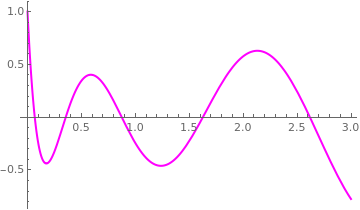
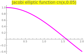
Example 19: Let us consider the Jacobi elliptic cosine function cn(x, k), which is a solution of the boundary value problem
|
Upon plotting the elliptic cosine function we determine an interval [1,2] containing its zero.
Plot[JacobiCN[x, 1/20], {x, 0, 2},
PlotStyle -> {Thickness[0.01], Magenta},
PlotLabel ->
Style["Jacobi elliptic function cn(x,0.05)", FontSize -> 16,
Background -> Yellow]]
|
|
| Jacobi elliptic cosine function cn(-x,0.05). | Mathematica code |
First, we find its root using the standard Mathematica command
f1[x_] = D[JacobiCN[x, 1/20], x];
If we apply the Chebyshev iteration scheme, we need four iterations to obtain the same accuracy:
ChebyshevMethodList[f[x], {x, 1}, 4]
Re[%]
Re[%]
- Gautschi, Walter, "Alexander M. Ostrowski (1893–1986): His life, work, and students", can be downloaded from http://www.cs.purdue.edu/homes/wxg/AMOengl.pdf.
- Grau-Sánchez, M., Grau, A., Noguera, M., "Ostrowski type methods for solving systems of nonlinear equations," Applied Mathematics and Computation, 2011, Vol. 218, pp. 2377–2385.
- Shammas, N., Ostrowski’s Method for Finding Roots
IX. Muller’s Method
Muller’s method is a generalization of the secant method, in the sense that it does not require the derivative of the function. Muller's method finds a root of the equation \( f(x) =0 . \) It is an iterative method that requires three starting points \( \left( p_0 , f(p_0 ) \right) , \ \left( p_1 , f(p_1 ) \right) , \ \left( p_2 , f(p_2 ) \right) . \) A parabola is constructed that passes through the three points; then the quadratic formula is used to find a root of the quadratic for the next approximation. If the equation f(x) = 0 has a simple root, then it has been proved that Muller’s method converges faster than the secant method and almost as fast as Newton’s method. The method can be used to find real or complex zeros of a function and can be programmed to use complex arithmetic.
David Eugene Muller (1924--2008) was a professor of mathematics and computer science at the University of Illinois (1953–1992), when he became an emeritus professor, and was an adjunct professor of mathematics at the New Mexico State University (1995-2008). Muller received his BS in 1947 and his PhD in 1951 in physics from Caltech; an honorary PhD was conferred by the University of Paris in 1989. He was the inventor of the Muller C-element (or Muller C-gate), a device used to implement asynchronous circuitry in electronic computers. He also co-invented the Reed–Muller codes.
Without loss of generality, we assume that p2 is the best approximation to the root and consider the parabola through the three starting values. Make the change of variable
If Muller’s method is used to find the real roots of \( f(x) =0 , \) it is possible that one may encounter complex approximations, because the roots of the quadratic in \( at^2 + bt +c =0 \) might be complex (nonzero imaginary components). In these cases the imaginary components will have a small magnitude and can be set equal to zero so that the calculations proceed with real numbers.
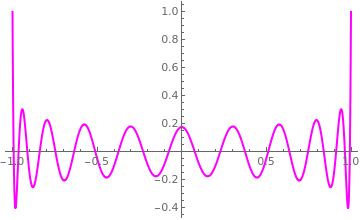
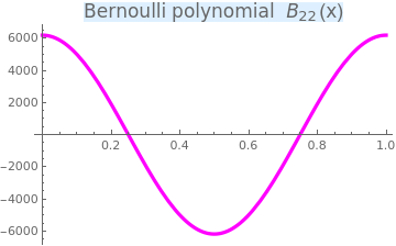
Example 20: We consider the Bernoulli polynomial of order n:
|
Upon plotting the Bernoulli polynomial we determine an interval [0.1, 0.5] containing its zero.
Plot[{BernoulliB[22, x]}, {x, 0, 1},
PlotStyle -> {Thickness[0.01], Magenta}, PlotLabel -> Style["Bernoulli polynomial \!\(\*SubscriptBox[\(B\), \ \(22\)]\)(x)", FontSize -> 16, Background -> LightBlue]] |
|
| Bernoulli polynomial of order 22. | Mathematica code |
First, we pick up three points (x1, y1), (x2, y2), and (x3, y3), where
- Brent, R.P., An algorithm with guaranteed convergence for finding a zero of a function, Computer Journal, 1971, Vol. 14, Issue 4, pp. 422-425.
- Bus, J. C. P., and T. J. Dekker, Two efficient algorithms with guaranteed convergence for finding a zero of a function, ACM Transactions on Mathematical Software (TOMS), 1.4 (1975): 330-345.
- Chun, C., Ham, Y.M., Some fourth-order modifications of Newton’s method, Applied Mathematics and Computation, 2008, Vol. 197, pp. 654--658.
- Dekker, T.J., Finding a zero by means of successive linear interpolation, Constructive Aspects of the Fundamental Theorem of Algebra, B. Dejon and P. Henrici, Eds., Wiley Interscience, London, 1969, pp. 37--51.
- Feng, X.L., He, Y.N., High order iterative methods without derivatives for solving nonlinear equations, Applied Mathematics and Computation, 2007, Vol. 186, pp. 1617--1623.
- Jarratt, P., Some fourth order multipoint iterative methods for solving equations, Math. Comput. 20 (95) (1966) 434–437.
- King, R.F., A Family of Fourth Order Methods for Nonlinear Equations, SIAM Journal on Numerical Analysis, 1973, Volume 10, Issue 5, pp. 876--879. https://doi.org/10.1137/0710072
- Kou, J., Li, Y., The improvements of Chebyshev–Halley methods with fifth-order convergence, Applied Mathematics and Computation, 2007, Volume 188, Issue 1, pp. 143--147. https://doi.org/10.1016/j.amc.2006.09.097
- Kung, H.T., Traub, J.F., Optimal order of one-point and multipoint iteration, Journal of the Association for Computing Machinery (ACM), 1974, Vol. 21, No. 4, pp. 643--651. https://doi.org/10.1145/321850.321860
- Muller, D.E., A method for solving algebraic equations using automatic computer, Mathematical Tables and other Aids to Computation, 1956, Vol. 10, No. 56, pp. 208--215.
- Ostrowski, A.M., Solution of Equations in Euclidean and Banach Space, Academic Press, New York, 1973.
- Parhi, S.K., Gupta, D.K., A sixth order method for nonlinear equations, Applied Mathematics and Computation, 2008, Vol. 203, pp. 50--55.
- Traub. J.F., Iterative Methods for the Solution of Equation, American Mathematical Society; Second Edition (January 1, 1982) New Jersy.
- Wang, X., Kou, J., Li, Y., A variant of Jarratt method with sixth-order convergence, Applied Mathematics and Computation, 2008, Vol. 204, pp. 14--19.
Return to Mathematica page
Return to the main page (APMA0330)
Return to the Part 1 (Plotting)
Return to the Part 2 (First Order ODEs)
Return to the Part 3 (Numerical Methods)
Return to the Part 4 (Second and Higher Order ODEs)
Return to the Part 5 (Series and Recurrences)
Return to the Part 6 (Laplace Transform)
Return to the Part 7 (Boundary Value Problems)